Hamiltonian Monte Carlo

In the previous two posts in this series, we built up enough background material in physics to re-derive Hamilton’s equations. We now ready for Hamiltonian Monte Carlo (HMC) (Duane et al., 1987), a Markov chain Monte Carlo (MCMC) algorithm that improves on a random walk using Hamiltonian dynamics. Now that we understand Hamiltonian dynamics, understanding HMC is relatively easy.

I assume the reader is familiar with the material and notation in the previous two posts, and is at least familiar with the Metropolis–Hastings (MH) algorithm. I’ll review MH next, but if any details do not make sense, see my MH post.

Correlated Metropolis steps

In Bayesian inference, we often want to sample from a posterior density $p(\boldsymbol{\theta} \mid \mathbf{X})$ where $\boldsymbol{\theta}$ are our model parameters and $\mathbf{X}$ is our data. The Metropolis–Hastings algorithm (Metropolis et al., 1953; Hastings, 1970) walks an implicit Markov chain whose stationary distribution is $p(\boldsymbol{\theta} \mid \mathbf{X})$, meaning that once the Markov chain has mixed, each state is a sample from the posterior.

Metropolis–Hastings works because, given a transition kernel $k(\cdot)$ that computes a transition probability $k(\boldsymbol{\theta} \mapsto \boldsymbol{\theta}^{\prime})$, any Markov process will converge to a unique stationary distribution $\pi(\boldsymbol{\theta})$ provided it is ergodic and satisfies the detailed balance,

$\pi(\boldsymbol{\theta}) k(\boldsymbol{\theta} \mapsto \boldsymbol{\theta}^{\prime}) = \pi(\boldsymbol{\theta}^{\prime}) k(\boldsymbol{\theta}^{\prime} \mapsto \boldsymbol{\theta}). \tag{1}$

Ensuring the Markov process is ergodic is straightforward: we can avoid periodicity by ensuring the probability of staying on any state is nonzero, and we can ensure a single recurrent class by picking a proposal distribution such that there is a nonzero probability of jumping to any point in parameter space. However, ensuring the detailed balance in $(1)$ requires an acceptance criteria. Let $\boldsymbol{\theta}^{\prime} \sim q(\boldsymbol{\theta})$ be some function for proposing candidate jumps in the Markov process. If we accept its proposals with probability $\alpha(\boldsymbol{\theta} \mapsto \boldsymbol{\theta}^{\prime})$ where,

$\alpha(\boldsymbol{\theta} \mapsto \boldsymbol{\theta}^{\prime}) = \min\Big\{1, \frac{ \pi(\boldsymbol{\theta}^{\prime}) k(\boldsymbol{\theta}^{\prime} \mapsto \boldsymbol{\theta}) }{ \pi(\boldsymbol{\theta}) k(\boldsymbol{\theta} \mapsto \boldsymbol{\theta}^{\prime}) } \Big\}, \tag{2}$

then we ensure the detailed balance holds for $k(\cdot)$. In Bayesian inference, we set $\pi(\boldsymbol{\theta}) = p(\boldsymbol{\theta} \mid \mathbf{X})$, and we sample from our posterior by walking the Markov chain until it mixes. If the transition kernel is symmeteric, meaning $k(\boldsymbol{\theta} \mapsto \boldsymbol{\theta}^{\prime}) = k(\boldsymbol{\theta}^{\prime} \mapsto \boldsymbol{\theta})$, then Metropolis–Hastings reduces to the Metropolis algorithm with acceptance criteria,

$\alpha(\boldsymbol{\theta} \mapsto \boldsymbol{\theta}^{\prime}) = \min\Big\{1, \frac{ \pi(\boldsymbol{\theta}^{\prime}) }{ \pi(\boldsymbol{\theta}) } \Big\}. \tag{3}$

A challenge with both the Metropolis–Hastings and Metropolis algorithms is that the proposed state $\boldsymbol{\theta}^{\prime}$ is correlated with the current state $\boldsymbol{\theta}$. For example, in a simple Gaussian random walk, the proposal is just the previous state with additive Gaussian noise. Increasing the MH step size does not necessarily help, because bigger proposed jumps in parameter space may result to a higher rejection rate in $(2)$ or $(3)$. This becomes even more problematic if $\boldsymbol{\theta}$ is high-dimensional. While we have asymptotic guarantees, we often can’t rely on them in practice, i.e. MH can be very, very slow to converge.

Hamiltonian Monte Carlo

HMC leverages Hamiltonian dynamics to propose a new state $\boldsymbol{\theta}^{\prime}$ that is both uncorrelated with the previous state and has a high probability of being accepted. Imagine that our parameters $\boldsymbol{\theta} = [\theta_1 \dots \theta_K]^{\top}$ are the generalized coordinates, a $K$-dimensional position vector, in a fictitious physical system, and let’s introduce auxiliary generalized momenta $\mathbf{r} = [r_1 \dots r_K]^{\top}$. By fiat, let’s say that the Hamiltonian of our fictitious physical system is equal to the log joint distribution on $(\mathbf{r}, \boldsymbol{\theta})$:

$\begin{aligned} H(\mathbf{r}, \boldsymbol{\theta}) &\triangleq - \log p(\mathbf{r}, \boldsymbol{\theta} \mid \mathbf{X}) \\ &= - \log p(\mathbf{r}) - \log p(\boldsymbol{\theta} \mid \mathbf{X}) \\ &= T(\mathbf{r}) + V(\boldsymbol{\theta}). \end{aligned} \tag{4}$

Here, we have defined kinetic energy as $T(\mathbf{r}) \triangleq -\log p(\mathbf{r})$ and potential energy as $V(\boldsymbol{\theta}) \triangleq -\log p(\boldsymbol{\theta} \mid \mathbf{X})$. The second equality holds because we assume $\mathbf{r}$ is independent of $\boldsymbol{\theta}$.

Now consider the following MCMC algorithm. On each sampling step, randomly resample the momentum variables $\mathbf{r}$ from a spherical Gaussian distribution,

$\mathbf{r} \sim \mathcal{N}_K(\mathbf{0}, \mathbf{M}), \tag{5}$

and then update both $\mathbf{r}$ and $\boldsymbol{\theta}$ by simulating Hamiltonian dynamics using Hamilton’s equations:

$\begin{aligned} \frac{\text{d}\theta_k}{\text{d}t} &= \frac{\partial H}{\partial r_k}, \\ \frac{\text{d}r_k}{\text{d}t} &= -\frac{\partial H}{\partial \theta_k}. \end{aligned} \tag{6}$

This would give us a new position vector $\boldsymbol{\theta}^{\prime}$ that is uncorrelated from the previous step $\boldsymbol{\theta}$. If the transition probabilities are symmetric and if Hamiltonian dynamics are volume-preserving—I’ll explain these qualifications later—, then we can accept this new proposal using the Metropolis criteria in $(3)$:

$\begin{aligned} \alpha((\mathbf{r}, \boldsymbol{\theta}) \mapsto (\mathbf{r}^{\prime}, \boldsymbol{\theta}^{\prime})) &= \min\Big\{1, \frac{p(\mathbf{r}^{\prime}, \boldsymbol{\theta}^{\prime} \mid \mathbf{X})}{p(\mathbf{r}, \boldsymbol{\theta} \mid \mathbf{X})} \Big\} \\ &= \min\Big\{1, \exp( \log p(\mathbf{r}^{\prime}, \boldsymbol{\theta}^{\prime} \mid \mathbf{X}) - \log p(\mathbf{r}, \boldsymbol{\theta} \mid \mathbf{X}) ) \Big\} \\ &= \min\Big\{1, \exp(- H(\mathbf{r}^{\prime}, \boldsymbol{\theta}^{\prime}) + H(\mathbf{r}, \boldsymbol{\theta})) \Big\}. \end{aligned} \tag{7}$

If we could simulate Hamiltonian dynamics exactly, the Hamiltonian $H$ would always be conserved exactly, and $(7)$ would always be $\min\{1, \exp(0)\} = 1$. As we will see, the main complication in implementing HMC is that we cannot simulate Hamiltonian dynamics exactly. Instead, we will use the leapfrog integrator, which approximates simulating the dynamics. However, if this approximation is good, then $H(\mathbf{r}^{\prime}, \boldsymbol{\theta}^{\prime}) - H(\mathbf{r}, \boldsymbol{\theta})$ should be small, and our acceptance rate will be high.

Note that above, we’ve only shown that $p(\mathbf{r}, \boldsymbol{\theta} \mid \mathbf{X})$ is the stationary distribution of our Markov process. However, at least intuitively, the probability of transitioning from $\boldsymbol{\theta}$ to $\boldsymbol{\theta}^{\prime}$ also satisfies the detailed balance because we resample $\mathbf{r}$ from a distribution that is independent of $\boldsymbol{\theta}$. In fact, this intuition is correct, meaning we are also sampling from the stationary distribution $p(\boldsymbol{\theta} \mid \mathbf{X})$. See Duane’s original paper for a proof.

HMC is a very clever idea. If our approximation of Hamiltonian dynamics is good, then we can make possibly large, uncorrelated jumps in parameter space while having a high probability of acceptance because the difference in $(7)$ is often small.

Now that we understand the big picture, we need to discuss three details: $1)$ Are the transition probabilites symmetric? $2)$ Are Hamiltonian dynamics volume-preserving? $3)$ How can we simulate Hamiltonian dynamics? Let’s take a look at each of these points separately.

Time reversal symmetry

The correctness HMC depends on the proposal distribution being symmetric. To understand why this symmetry holds, we need to understand that Hamilton’s equations are invariant under a reversal in the direction of time, where $t \rightarrow -t$. Or Hamilton’s equations are reversible. While the position vector $\boldsymbol{\theta}$ does not depend on time, momenta $\mathbf{r}$ does through velocity, and is therefore also reversed:

$r_k = m_k v_k = m_k \frac{\text{d}\theta_k}{\text{d}t} \rightarrow m_k \frac{\text{d}\theta_k}{\text{d}(-t)} = -r_k. \tag{8}$

Above, $m_k$ and $v_k$ are the mass and velocity associated with the $k$-th parameter. Plugging $t \rightarrow -t$ and $r_k \rightarrow -r_k$ into $(3)$, we get:

$\begin{aligned} \frac{\text{d}\theta_k}{\text{d}(-t)} &= -\frac{\partial H}{\partial r_k}, \\ \frac{\text{d}(-r_k)}{\text{d}(-t)} &= -\frac{\partial H}{\partial \theta_k}. \end{aligned} \tag{9}$

In other words, the forms of the equations don’t change from $(6)$. The physical interpretation is that if we allow a physical system to evolve up to time $t$, then flip the sign of each particle’s velocity, and then allow the system to evolve again for another time interval $t$, the system would return to its original state. Put differently, if we observe a system evolve through time—a bird flying from ground to branch—it is impossible to know a priori if we are observing the forward- or backward-in-time evolution because the system has time reversal symmetry. In physics, this leads to concepts such as Loschmidt’s paradox and the arrow of time.

HMC ensures the proposal distribution is symmetric with this trick: after each sampling step, flip the sign of the momenta variable, so $\mathbf{r}_t = - \mathbf{r}_t$ on iteration $t$. On half of the steps, we move forward in time; and on the other half, we move backwards in time. That said, this is not needed in practice if we sample the momenta from a symmetric distribution such as $(5)$ because positive or negative mometum components (each $r_k$) are equally likely.

There is one caveat to this discussion. We aren’t simulating Hamiltonian dynamics exactly, and therefore the leapfrog integrator mentioned previously must also be symmetric. We’ll see that it is.

Volume presevation

A second important property of Hamilton’s equations is that they are volume-preserving transformations. Why does this matter? To be frank, I haven’t seen a single resource that explains this point well, although (Neal, 2011) implies the answer when he writes:

If we proposed new states using some arbitrary, non-Hamiltonian, dynamics, we would need to compute the determinant of the Jacobian matrix for the mapping the dynamics defines, which might well be infeasible.

Let me explain what he means in more detail.

At each sampling step, we’re applying a deterministic transformation to the parameters and momenta. Let’s call this transformation $\Phi(\mathbf{r}, \boldsymbol{\theta}) \mapsto (\mathbf{r}^{\prime}, \boldsymbol{\theta}^{\prime})$. How do we know we’re still sampling from the desired joint distribution after applying this transformation? In probability, there is a simple solution: apply a change of variables:

Let $\mathbf{x}$ be a $K$-dimensional random variable with a joint density $f_X$. If $\mathbf{y} = h(\mathbf{x})$ where $h$ is an invertible, differentiable function, then $\mathbf{y}$ has density $f_Y$:

$f_Y(\mathbf{y}) = f_X(h^{-1}(\mathbf{y})) \big| \text{det}(\nabla_{\mathbf{y}} h^{-1}(\mathbf{y})) \big|.$

Here, the term $\nabla_{\mathbf{y}} h^{-1}(\mathbf{y})$ is the Jacobian of the inverse of the transformation $h$. In our case, this means that the Metropolis acceptance ratio in $(7)$ can be written more explicitly as

$\min\!\Big\{1, \exp\!\big(- H(\Phi^{-1}(\mathbf{r}^{\prime}, \boldsymbol{\theta}^{\prime})) + H(\mathbf{r}, \boldsymbol{\theta}) \big) \big| \text{det}\big( \nabla_{\mathbf{r}^{\prime}, \boldsymbol{\theta}^{\prime}} \Phi^{-1}(\mathbf{r}^{\prime}, \boldsymbol{\theta}^{\prime}) \big) \big| \Big\}. \tag{10}$

The reason no one writes this out in HMC is because the invertible and differentiable transformation $\Phi$ is Hamiltonian dynamics, and the determinant of a voluming-preserving transformation is one. For a geometric intuition of the determinant, see my previous post on determinantal point processes. So volume preservation means we do not have to write the Metropolis acceptance ratio as in $(10)$ and can instead write it as in $(7)$.

I haven’t seen a simple, standalone proof of the fact that Hamiltonian dynamics are volume-preserving, and I suspect this is why Neal just proves directly that the determinant of the transformation is one, a sufficient claim for our purposes and one that requires less knowledge about statistical mechanics. I won’t include his proof here because I don’t think it adds to our intuition at this point.

Once again, we have a caveat. Since we aren’t simulating Hamiltonian dynamics exactly, the leapfrog integrator mentioned previously must also be volume-preserving. Again, we’ll see that it is.

Leapfrog integration

Our remaining question is: how can we simulate Hamiltonian dynamics? This is an important problem in physics, and there are many algorithms for doing so. For example, here is a textbook on the topic and here is a recent paper. The class of methods for providing numerical solutions to Hamilton’s equations are symplectic integrators, where symplectic refers to a type of manifold. Without getting sidetracked, the main idea is that the generalized momenta and position $(\mathbf{r}, \boldsymbol{\theta})$ live on a symplectic manifold, and symplectic integrators are integrators whose solutions are on symplectic manifolds. Because these integrators assume the right structure for the problem, they are better at long-term integration because they do not accumulate systematic error. You can find many examples of this systematic error for simpler integrators, for example in this blog post by Colin Carroll, this StackExchange post, and of course (Neal, 2011).

Symplectic integration is a complex topic, and the main point is just that the leapfrog integrator is a specific instance of a general set of solutions that is particularly convenient for HMC. In the original paper, Duane lists three reasons for choosing the leapfrog integrator:

1. It is simple.
2. It ensures exact reversibility.
3. It preserves volume.

The first reason is just nice-to-have. The second point ensures the correctness of HMC, and the third point makes our calculations tractable, since we can ignore the Jacobian of our transformation.

The method is called the leapfrog integrator or the leapfrog method because it discretizes time using a small stepsize $\varepsilon$, computing a half-step update of momenta, a full-step update of position using the new momenta, and finally another half-step update in momenta using the new position:

$\begin{aligned} r_k^{(t + \varepsilon/2)} &= r_k^{(t)} - (\varepsilon/2) \frac{\partial V}{\partial \theta_k}(\boldsymbol{\theta}^{(t)}), \\ \theta_k^{(t + \varepsilon)} &= \theta_k^{(t)} + \varepsilon \frac{r_k^{(t + \varepsilon/2)}}{m_k}, \\ r_k^{(t + \varepsilon)} &= r_k^{(t + \varepsilon/2)} - (\varepsilon/2) \frac{\partial V}{\partial \theta_k}(\boldsymbol{\theta}^{(t + \varepsilon)}). \end{aligned} \tag{11}$

We can imagine the momenta and position estimates leapfrog jumping over each other. Note that $\partial V / \partial \theta_k$ is just the gradient of the log likelihood, which we can compute using automatic differentation. This is why HMC is sometimes referred to as a gradient-based MCMC method.

Since we’re arbitrarily discretizing time into step sizes $\varepsilon$, we can run the leapfrog updates in $(11)$ as many times as we’d like to simulate a Metroplis jump using Hamiltonian dynamics. Both the number of steps and the step size $\varepsilon$ are hyperparameters, and tuning these hyperparameters is part of what makes HMC difficult in practice. See (Neal, 2011) for a detailed discussion of tuning HMC.

Example: Rosenbrock density

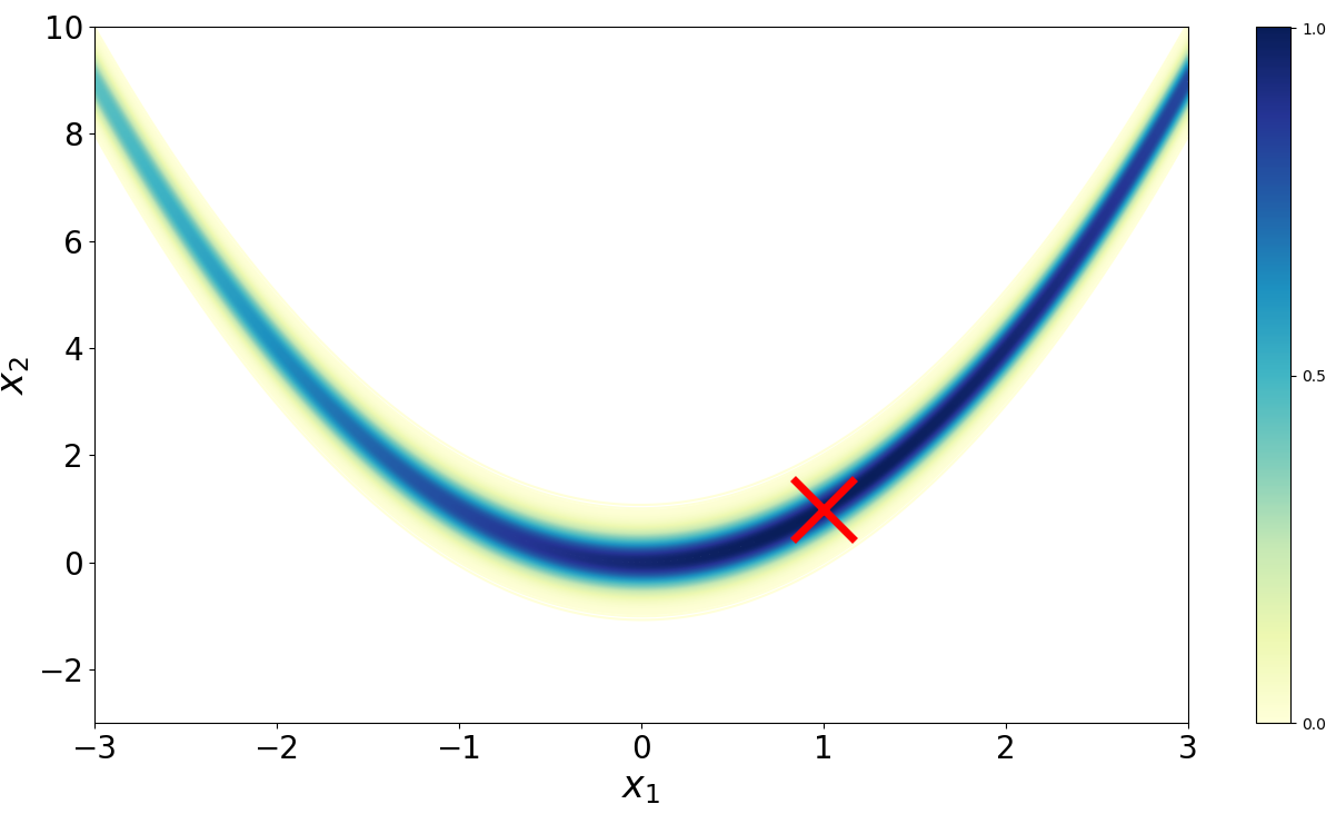
Imagine we want to sample from the Rosenbrock density (Figure $1$),

$p(x_1, x_2 \mid a, b) \propto \exp\Big\{-\frac{(a - x_1)^2 + b(x_2 - x_1^2)^2}{20}\Big\}. \tag{12}$

The Rosenbrock function (Rosenbrock, 1960) is a well-known test function in optimization because while finding a minimum is relatively easy, finding the global minimum at ($1$, $1$) is less trivial. (Goodman & Weare, 2010) adapted the function to serve as a benchmark for MCMC algorithms. I’ve also used this density to benchmark my implementation of Metroplis-Hastings

Figure 1. The Rosenbrock density (Equation $12$) with $a = 1$ and $b = 100$. Darker colors indicate higher probability. The global minimum is at $(x, y) = (a, a^2) = (1, 1)$ and denoted with a red "X".

Below is my implementation of Hamiltonian Monte Carlo run on the Rosenbrock density. I’ve used the autograd library to automatically differentiate the log density provided by the user. We can accept a proposed sample with probability $\alpha((\mathbf{r}, \boldsymbol{\theta}) \mapsto (\mathbf{r}^{\prime}, \boldsymbol{\theta}^{\prime}))$ by drawing a uniform random variable with support $[0, 1]$ and then checking if it is less than the acceptance criteria.

from   autograd import grad
import matplotlib.pyplot as plt
import numpy as np
from   scipy.stats import norm


def hmc(logp, n_samples, x0, n_steps, step_size):
    """Run Hamiltonian Monte Carlo to draw `n_samples` from the log density
    `logp`, starting at initial state `x0`.
    """
    momenta_dist = norm(0, 1)

    # Kinetic and potential energy functions.
    T = lambda r: -momenta_dist.logpdf(r).sum()
    V = lambda x: -logp(x)

    grad_V = grad(V)
    dim = len(x0)
    samples = np.empty((n_samples, dim))
    samples[0] = x0

    for i in range(1, n_samples):

        x_curr = samples[i-1]
        r_curr = momenta_dist.rvs(size=dim)
        x_prop, r_prop = leapfrog(x_curr, r_curr, n_steps, step_size, grad_V)

        H_prop = T(r_prop) + V(x_prop)
        H_curr = T(r_curr) + V(x_curr)
        alpha  = np.exp(-H_prop + H_curr)

        if np.random.uniform(0, 1) < alpha:
            x_curr = x_prop
        samples[i] = x_curr

    return samples


def leapfrog(x, r, n_steps, step_size, grad_V):
    """Run the leapfrog integrator forward `n_steps` using step size
    `step_size`.
    """
    x, r = x[:], r[:]
    for _ in range(n_steps):
        r = r - (step_size / 2) * grad_V(x)
        x = x + step_size * r
        r = r - (step_size / 2) * grad_V(x)
    return x, r


def log_rosen(x):
    """Compute the log of the Rosenbrock density.
    """
    return -((1 - x[0]) ** 2 + 100 * (x[1] - x[0] ** 2) ** 2) / 20


samples = hmc(
    logp=log_rosen,
    n_samples=1000,
    x0=np.random.uniform(low=[-3, -3], high=[3, 10], size=2),
    n_steps=20,
    step_size=0.03
)

plt.plot(samples[:, 0], samples[:, 1])
plt.show()

That’s it. Despite its conceptual depth, Hamiltonian Monte Carlo is, like Metropolis–Hastings, surprisingly simple to implement. This code could easily be amended to support burn in, multiple chains, and so forth, but it is the minimal code required to understand the algorithm.

Figure 2. Three randomly initialized Markov chains run on the Rosenbrock density (Equation $4$) using HMC. The global minimum is at $(x, y) = (a, a^2) = (1, 1)$ and denoted with a black "X".

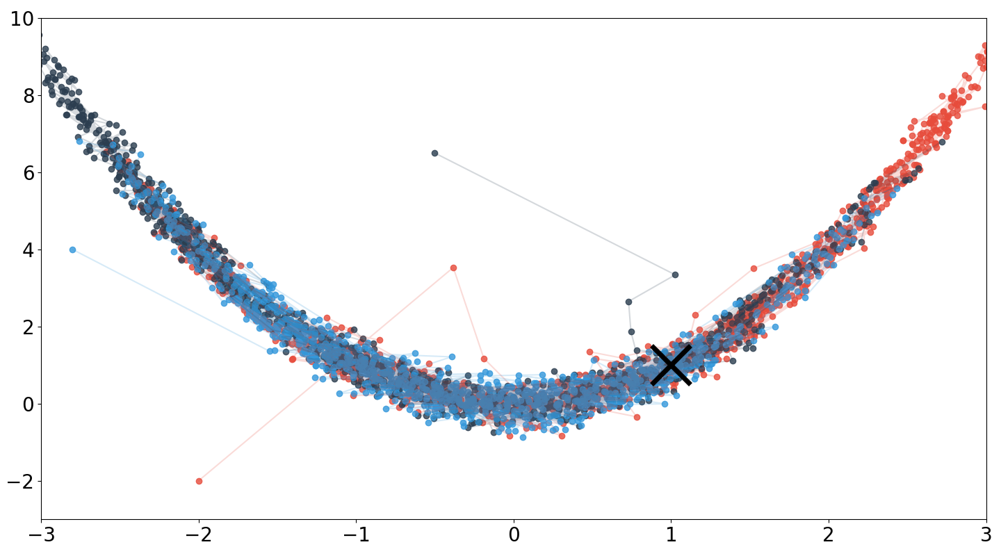
The above code is the basis for Figure $2$, which runs three Markov chains from randomly initialized starting points. A few points are worth mentioning when comparing this result to my MH result. First, notice that HMC jumps to the high probability areas much faster than MH. This is probably because HMC leverages the gradient of the log density. Second, notice that HMC explores the Rosenbrock density more thoroughly given the same number of iterations ($1000$). Finally, HMC accepted nearly all of the proposals ($\sim\!99\%$) because the leapfrog integrator could well-approximate the dynamics for this simple problem.

Conclusion

Hamiltonian Monte Carlo, like Metropolis–Hastings, is a beautifully simple algorithm given a basic understanding of MCMC and Hamiltonian dynamics. Rather than performing a random walk, HMC introduces auxiliary momenta variables that allow us to simulate a fictitious physical system using Hamiltonian dynamics. This simulation creates MCMC jumps with less correlation between states, and if the approximated dynamics are good, can result in a very high acceptance rate.