The Euler–Lagrange Equation

Originally proposed by (Duane et al., 1987), Hybrid Monte Carlo is a Metropolis–Hastings algorithm in which each step is chosen according to the energy in a simulated Hamiltonian dynamical system. This method is now called Hamiltonian Monte Carlo, and the acronym “HMC” remains unchanged. The advantage of HMC is that it can propose distance states that still have high probabilities of being accepted. It is a popular choice over a Gaussian random walk, which may converge more slowly. However, understanding HMC depends on understanding the Hamiltonian reformulation of classical mechanics. While (Neal, 2011) and (Betancourt, 2017) are excellent introductions to HMC, they both expect the reader to already understand Hamilton’s equations. In my mind, Hamiltonian mechanics is the conceptual linchpin that gives any intuition for why the method works. My goal is to bridge this conceptual gap. I hope this is useful for others who are interested in HMC but lack a sufficient background in physics.

This is the first post in a three-part series. In this post, I will frame and motivate the problem that the Euler–Lagrange equation solves, finding the stationary function of a functional. This class of problems is called the calculus of variations. In the next post, I will explain how Lagrangian and Hamiltonian mechanics use the Euler–Lagrange equation to reformulate of Newtonian mechanics. The basic idea will be to reformulate classical mechanics, which models a system of particles by specifying all the system’s forces, as a model in which the total energy is conserved. Finally, in the last post, I will discuss Hamiltonian dynamics in the context of HMC.

With this outline in mind, let’s start with the calculus of variations.

An example of a variational problem

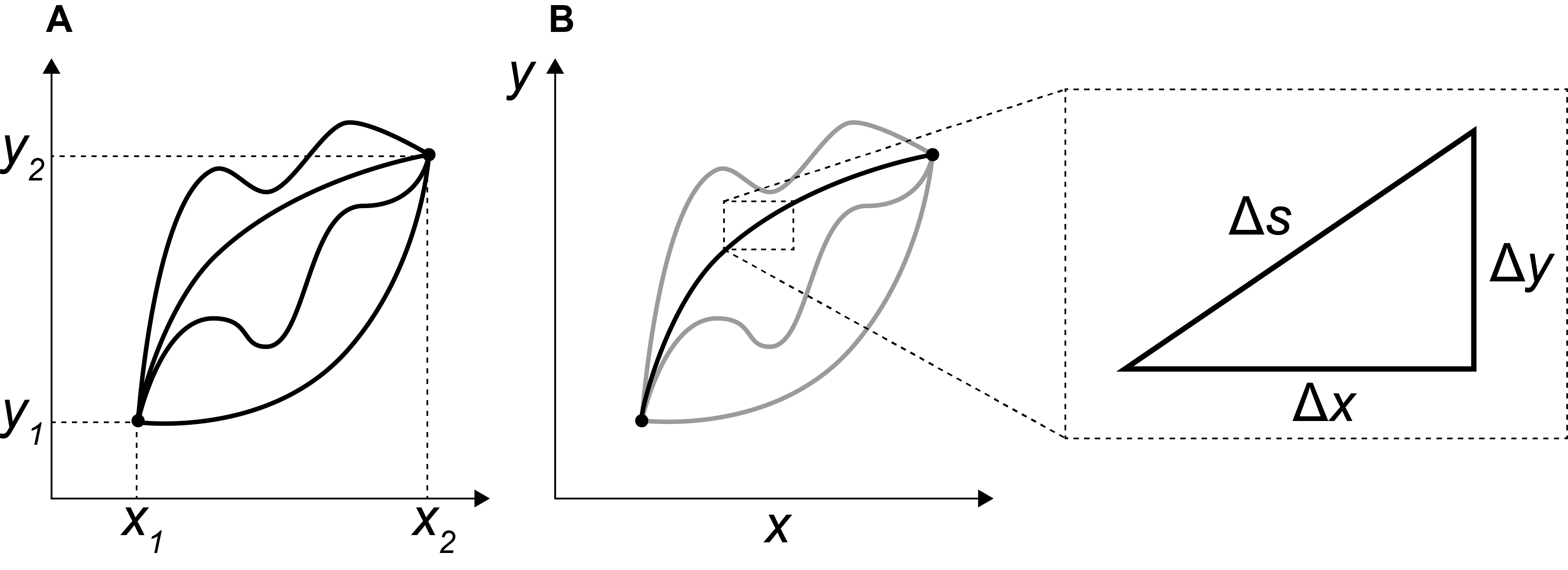
Let’s introduce the calculus of variations through an example. What is the shortest path between two points on a plane, $(x_1, y_1)$ and $(x_2, y_2)$? We may intuit that the answer is a straight line, but there are an infinite number of such paths. Can we prove it? One way to formalize the problem is to consider all functions described by the equation

$y = f(x), \quad x_1 \leq x \leq x_2, \tag{1}$

subject to the constraint that

$f(x_1) = y_1, \quad f(x_2) = y_2. \tag{2}$

In words, the function can be arbitrarily curved, but it must be fixed at the endpoints (Figure $1\text{A}$). We will see that $f$ also needs to be continuously differentiable. If we imagine zooming in on a single path (Figure $1\text{B}$), we can approximate a finite but very small segments along that path as $\Delta s$ where

$\Delta s \approx \sqrt{(\Delta x)^2 + (\Delta y)^2}, \tag{3}$

by the Pythagorean theorem. This suggests an infinitesimal representation in terms of the derivative of the function $f$,

$\text{d}s = \sqrt{(\text{d}x)^2 + (\text{d}y)^2} = \sqrt{1 + (y^{\prime})^2} \,\text{d}x. \tag{4}$

In words, $(4)$ is the infinitesimal distance traveled by infinitesimal changes in the $(x, y)$-coordinates as quantified by the first derivative $y^{\prime}$. The total length of the path is given by integrating $(4)$ between the two endpoints,

$S = \int_{x_1}^{x_2} \sqrt{1 + (y^{\prime})^2} \,\text{d}x. \tag{5}$

Finding the shortest path is equivalent to finding the solution of the following minimization problem: among all functions $(1)$ that satisfy the contraint $(2)$, find the one which minimizes $(5)$.

Figure 1. (A) Many paths between two points, $(x_1, y_1)$ and $(x_2, y_2)$. (B) A linear approximation of a small but finite section of a possibly curved line.

The integrated term in $(5)$ is called a functional. If every number $x$ in a set $\mathcal{X}$ corresponds to a number $y$, we say there is defined on the set $\mathcal{X}$ a function $y = f(x)$ and that $\mathcal{X}$ is its domain. A functional is a natural generalization of this concept where $\mathcal{X}$ is a set of mathematical objects of any kind. Thus, a generalization of $(5)$ is

$S = \int_{x_1}^{x_2} F(x, y, y^{\prime}, \dots) \,\text{d}x. \tag{6}$

This notation means that the functional $F$ may have an explicit dependence on $x$, in addition to the implicit dependencies through $y$, $y^{\prime}$, and so forth. In our example, the functional only depends on $y^{\prime}$.

Since maximizing $F(x)$ is equivalent to minimizing $-F(x)$, the distinction between maxima and minima is not interesting for functionals, and without loss of generality we focus on minimization. In our case, $F$ outputs distance, and therefore minimizing the integral minimizes total distance. However, if $F$ were an expression of time, then minimizing $F$ would represent minimizing total time. For example, Fermat’s principle, also called the principle of least time, states that the path a ray takes between two points minimizes total time. The Brachistochrone curve is the curve of fastest descent, assuming a frictionless surface and a uniform gravitional field.

These types of problems can all be solved using the calculus of variations. In elementary calculus, a function is stationary when its derivative is zero at a point $x_0$, meaning it attains a minimum or maximum. In the calculus of variations, a functional is stationary for a particular function $f_0$ when it attains a minimum or maximum.

According to (Aleksandrov et al., 1999), this branch of mathematics became important after connections were made to many problems in physics and classical mechanics. This is because, as we will see, a function that is the stationary function of a functional must satisfy a certain differential equation, the Euler–Lagrange equation; and many problems in physics take the form of differential equations. Thus, the calculus of variations is fascinating because the most famous problems in the field seem to suggest that nature often “knows” to take the most efficient path. This is called the variational principle.

The Euler–Lagrange equation

In calculus, a necessary condition for an extremum of a differentiable function $f$ at a point $x_0$ is that $f^{\prime}(x_0) = 0$. This is easy to visualize: at the top of a hill or the bottom of a valley, a line tangent to the curve is horizontal. Equivalently, the differential of $f$ must be zero: $\text{d}f = f^{\prime}(x_0) \text{d}x = 0$. The Euler–Lagrange equation will make a statement that is analogous to $\text{d}f = 0$ but for functionals rather than functions. This is a powerful result because it allows us to exclude any function that does not satisfy this criteria from having extrema.

Given a function $F(x, y, y^{\prime})$, the simplest integral in the calculus of variations, what is the extremum value

$I(y) = \int_{x_1}^{x_2} F(x, y, y^{\prime}) \text{d}x? \tag{7}$

To answer this question, we will use a simple but clever idea. Imagine we have a function $\bar{y}(x)$ that has the same endpoints as $y(x)$ but is otherwise possibly offset,

$\bar{y}(x) = y(x) + \varepsilon \delta(x), \tag{8}$

Let $\varepsilon$ be an arbitrary value. Then we need the constraint

$\delta(x_1) = \delta(x_2) = 0. \tag{9}$

This constraint ensures that the functions $\bar{y}(x)$ and $y(x)$ share endpoints regardless of the value of $\varepsilon$ or the shape of $\delta(x)$ (Figure $2$). Furthermore, we assume that $\delta$ is continuously differentiable. The term $\varepsilon$ is called the variational parameter; note that as $\varepsilon \rightarrow 0$, the original function $y(x)$ is recovered from $\bar{y}(x)$.

Figure 2. Illustration of equation $(8)$. An infinite number of functions can be represented as $\bar{y}(x)$, offset on the $y$-axis by $\eta(x)$.

Let’s take the derivative of $(8)$ with respect to the $\varepsilon$ evaluated at zero, set that derivative equal to zero, and then simply. The resulting expression will be the Euler–Lagrange equation, a second-order partial differential equation that expresses the function $y$ in terms of its extremum or the stationary point for the functional $F$ in $(7)$.

First, let’s take the derivatives of $\bar{y}$ and $\bar{y}^{\prime}$ with respect to $\varepsilon$:

$\begin{aligned} \frac{\partial \bar{y}}{\partial \varepsilon} &= \delta(x). \\ \frac{\partial \bar{y}^{\prime}}{\partial \varepsilon} &= \frac{\partial}{\partial \varepsilon} \left(y^{\prime}(x) + \varepsilon \delta^{\prime}(x) \right) = \delta^{\prime}(x). \end{aligned} \tag{10}$

Next, taking the derivative of $(7)$ evaluated at $\varepsilon = 0$ and setting it equal to zero, we get

$\begin{aligned} \frac{\text{d}I}{\text{d}\varepsilon}\Bigg|_{\varepsilon=0} &= \int_{x_1}^{x_2} \left[\frac{\partial F}{\partial \bar{y}} \frac{\partial \bar{y}}{\partial \varepsilon} + \frac{\partial F}{\partial \bar{y}^{\prime}} \frac{\partial \bar{y}^{\prime}}{\partial \varepsilon} \right] \text{d}x \\ &= \int_{x_1}^{x_2} \left[\frac{\partial F}{\partial \bar{y}} \delta(x) + \frac{\partial F}{\partial \bar{y}^{\prime}} \delta^{\prime}(x) \right] \text{d}x \\ &= \int_{x_1}^{x_2} \frac{\partial F}{\partial \bar{y}} \delta(x) \text{d}x + \int_{x_1}^{x_2} \frac{\partial F}{\partial \bar{y}^{\prime}} \delta^{\prime}(x) \text{d}x. \end{aligned} \tag{11}$

Now we can use integration by parts for the rightmost integral:

$\begin{aligned} v^{\prime} &= \delta^{\prime}(x) & u &= \frac{\partial F}{\partial \bar{y}^{\prime}} \\ v &= \delta(x) & u^{\prime} &= \frac{\text{d}}{\text{d}x} \Big(\frac{\partial F}{\partial \bar{y}^{\prime}}\Big). \end{aligned} \tag{12}$

Note that based on $(8)$, when we set $\varepsilon = 0$, then $\bar{y} = y$. Giving us

$\begin{aligned} 0 &= \frac{\text{d}I}{\text{d}\varepsilon}\Bigg|_{\varepsilon=0} \\ 0 &= \int_{x_1}^{x_2} \frac{\partial F}{\partial y} \delta(x) \text{d}x + \int_{x_1}^{x_2} \frac{\partial F}{\partial y^{\prime}} \delta^{\prime}(x) \text{d}x \\ 0 &\stackrel{\star}{=} \int_{x_1}^{x_2} \frac{\partial F}{\partial y} \delta(x) \text{d}x + \cancel{\frac{\partial F}{\partial y^{\prime}} \delta(x) \Bigg|_{x_1}^{x_2}} - \int_{x_1}^{x_2} \frac{\text{d}}{\text{d}x} \Big(\frac{\partial F}{\partial y^{\prime}}\Big) \delta(x) \text{d}x \\ 0 &= \int_{x_1}^{x_2} \frac{\partial F}{\partial y} \delta(x) \text{d}x - \int_{x_1}^{x_2} \frac{\text{d}}{\text{d}x} \Big(\frac{\partial F}{\partial y^{\prime}}\Big) \delta(x) \text{d}x \\ 0 &= \int_{x_1}^{x_2} \delta(x) \Big[ \frac{\partial F}{\partial y} - \frac{\text{d}}{\text{d}x} \Big(\frac{\partial F}{\partial y^{\prime}}\Big) \Big] \text{d}x. \end{aligned} \tag{13}$

The term on line $\star$ cancels because we assume that $\delta(x_1) = \delta(x_2)$. We want the above equation to be a minimum for any $\delta(x)$. This only holds when the bracketed term is zero or

$\frac{\partial F}{\partial y} - \frac{\text{d}}{\text{d}x} \Big(\frac{\partial F}{\partial y^{\prime}}\Big) = 0. \tag{14}$

This is the Euler–Lagrange equation. It is a second-order differential equation with respect to the function $y$. If $y(x)$ minimizes $I(y)$ in $(7)$, it must satsify $(14)$. This is analogous to the condition that $\text{d}f = 0$ in ordinary calculus.

The shortest distance

Armed with the Euler–Lagrange equation, let’s solve our example: what is the shortest distance between two points on a plane? Using the definition of $F$ in $(5)$, we want to solve $(17)$ for $y^{\prime}$. First, we know that the leftmost term in $(14)$ is zero or $\partial F / \partial y = 0$ because $F$ does not depend on $y$. Next, let’s solve the rightmost partial derivative in $(14)$:

$\begin{aligned} \frac{\partial F}{\partial y^{\prime}} &= \frac{1}{2} \left( 1 + (y^{\prime})^2 \right)^{-1/2} \cdot 2 y^{\prime} = \frac{y^{\prime}}{\sqrt{1 + (y^{\prime})^2}}. \end{aligned} \tag{15}$

Putting both results together, we get

$0 = \frac{\text{d}}{\text{d}x} \left( \frac{y^{\prime}}{\sqrt{1 + (y^{\prime})^2}} \right). \tag{16}$

Using the quotient rule, we get

$\begin{aligned} && 0 &= \frac{\text{d}}{\text{d}x} \left( \frac{y^{\prime}}{\sqrt{1 + (y^{\prime})^2}} \right) \\ \iff && 0 &= \frac{ (1 + (y^{\prime})^2)^{1/2} y^{\prime\prime} - y^{\prime} \frac{\text{d}}{\text{d}x} (1 + (y^{\prime})^2)^{1/2} }{ 1 + (y^{\prime})^2 } \\ \iff && 0 &= \frac{y^{\prime\prime}}{(1 + (y^{\prime})^2)^{1/2}} - \frac{(y^{\prime})^2 y^{\prime\prime}}{(1 + (y^{\prime})^2)^{3/2}} \\ \iff && 0 &= y^{\prime\prime} + (y^{\prime})^2 y^{\prime\prime} - (y^{\prime})^2 y^{\prime\prime} \\ \iff && 0 &= y^{\prime\prime}. \end{aligned} \tag{17}$

If $y^{\prime\prime} = 0$, then $y^{\prime}$ is a constant and $y$ is a straight line. Put conservely, $y$ must be a straight line to satisfy $(14)$, which is completely analogous to the calculus statement that a fixed point $x_0$ must satisfy the condition $f(x_0) = 0$. We have proven that the shortest distance between two points is a straight line.

Conclusion

The goal of this post was provide some intuition for and then derive the Euler–Lagrange equation in $(14)$. This is the foundational idea of the calculus of variations, which has many applications in physics. In the next post, we will use this variational framework to show how Newtonian mechanics can be reformulated into Lagrangian and Hamiltonian mechanics. We will introduce specific functions, called “Lagrangians”, that, when plugged into the Euler–Lagrange equation, reduce to Newton’s laws of motion. Rather than thinking about objects and forces across time, we will think about energy being conserved across time. This will provide good intuition for the final post on Hamiltonian Monte Carlo.

Acknowledgements

I thank Shivani Pandey and Federico Errica for reporting typos.