Modeling Repulsion with Determinantal Point Processes

A point process $\mathcal{P}$ over a set $\mathcal{X}$ is a probability measure over a random subset $X$ of $\mathcal{X}$. For example, in a Bernoulli point process with parameter $0 \leq p \leq 1$, each event $x \in X$ is independent and occurs with probability $p$. A determinantal point process (DPP) is a point process which is characterized by the determinant of a positive semi-definite matrix or kernel. The consequence of this is that DPPs are good for modeling repulsion, but why this follows from their definition may not be obvious. I want to explain my understanding of how they how they can be used as probabilistic models of repulsion. For simplicity, I only consider discrete sets.

It’s worth mentioning that while many point processes are determinantal, it is not well-understood why they are common (Tao, 2009), and they have recently received renewed attention in the mathematics and machine learning communities (Kulesza et al., 2012).

Determinantal point processes

A determinantal point process is a point process such that for every random subset $X$ drawn according to $\mathcal{P}$, we have for every subset $A \subseteq \mathcal{X}$:

$\mathcal{P}(A \subseteq X) = \det(K_A) \tag{1}$

where $K$ is a positive semi-definite (real, symmetric) matrix, called a kernel, indexed by the elements in $\mathcal{X}$ and,

$K_A \equiv [K_{ij}]_{i,j \in A}$

which means that the elements of $K$ are indexed by the indices of $A$. (We haven’t specified the actual values in $K$.) There is a lot of notation to unpack here. First, both $X$ and $A$ are subsets $\mathcal{X}$. But we say that $X$ is a random subset sampled according to $\mathcal{P}$. Thus, we call $X$ a realization of our point process, meaning it was sampled according to the distribution of $\mathcal{P}$, while $A$ is just any subset of $\mathcal{X}$. And for $\mathcal{P}$ to be a determinantal point process, a property of that realization must be that for every possible subset of points $A$, the probability of that set being in $X$ is equal to the determinant of some real, symmetric matrix. If you’re like me, what this means is not obvious, but it becomes more clear once we work through the math.

Let’s start with the simplest case. What happens when $A = \{x_i\}$. Then we have:

$\mathcal{P}(\{x_i\} \subseteq X) = K_{ii}$

In words, the diagonal of the matrix $K$ represents the marginal probability that $x_i$ is included in any realization $X$ of our determinantal point process $\mathcal{P}$. For example, if $K_{ii}$ is close to $1$, that means that any realization from the DPP will almost certainly include $x_i$. Now let’s look at a two element set, $A = \{x_i, x_j\}$:

$\begin{aligned} \mathcal{P}(\{x_i, x_j\} \subseteq X) &= \begin{vmatrix} K_{ii} & K_{ij} \\ K_{ji} & K_{jj} \end{vmatrix} \\ &= K_{ii} K_{jj} - K_{ij} K_{ji} \\ &= \mathcal{P}(\{x_i\} \subseteq X) \mathcal{P}(\{x_j\} \subseteq X) - K_{ij}^2 \end{aligned} \tag{1}$

where we can say $K_{ij}K_{ji} = K_{ij}^2$ because $K$ is symmetric. So the off-diagonal elements loosely represent negative correlation in the sense that the larger the value of $K_{ij}$, the less likely the joint probability of $\mathcal{P}(\{x_i, x_j\} \subseteq X)$.

If you’re like me, this above example from (Kulesza et al., 2012) is useful for two dimensions, but I find it hard to reason about how the probabilities change with higher-dimensional kernels. For example, this is the probability for three elements (dropping the set notation for legibility):

$\mathcal{P}(x_i, x_j, x_k) = \mathcal{P}(x_i) \mathcal{P}(x_j) \mathcal{P}(x_k) - \mathcal{P}(x_i) K_{jk}^2 - \mathcal{P}(_j) K_{ik}^2 - \mathcal{P}(x_k) K_{ij}^2 + 2 K_{ij} K_{jk} K_{ki}$

This is harder to reason about. I might note that if all the values are fixed and $K_{ij}$ increases, then $K_{ij}^2$ increases faster than $2 K_{ij}$, and therefore the probability decreases. But I find this kind of thinking about interactions slippery. I think an easier way to understand the determinantal point process is to use a geometrical understanding of the determinant while remembering that $K$ is symmetric.

Geometry of the determinant

Consider the geometrical intuition for the determinant of an $m \times n$ matrix: it is the signed scale factor representing how much a matrix transforms the volume of an $n$-cube into an $m$-dimensional parallelepiped. If that statement did not make sense, please read my previous post on a geometrical understanding of matrices. With this idea in mind, let’s consider the determinant for a simple matrix $M$:

$M = \begin{bmatrix} 1 & \beta \\ 0 & 1 \end{bmatrix}$

If we think of $M$ as a geometric transformation, then the columns of $M$ indicate where the standard basis vectors in $\mathbb{R}^2$ land in the transformed space. We can visualize this transformation by imagining how a unit square is transformed by $M$ (Figure $1$).

Figure 1: (Left) The unit cubed in $\mathbb{R}^2$ defined by standard basis vectors $\textbf{e}_1 = [1, 0]^{\top}$ and $\textbf{e}_2 = [0, 1]^{\top}$. (Right) The unit cube after being sheared by a matrix $M = \begin{bmatrix}1 & \beta \\ 0 & 1\end{bmatrix}$. The determinant of both matrices is $1$.

In this case, the determinant of $M$ is still $1$ because the area of the parallelogram (Figure $1b$) is the same as the area of the unit square (Figure $1a$). But what happens if $M$ were symmetric (Figure $2$)? Recall that symmetry is a property of DPP kernels.

Figure 2: (Left) The unit cubed in $\mathbb{R}^2$ defined by standard basis vectors $\textbf{e}_1 = [1, 0]^{\top}$ and $\textbf{e}_2 = [0, 1]^{\top}$. (Right) The unit cube after being sheared in both dimensions by a matrix $M = \begin{bmatrix}1 & \beta \\ \beta & 1\end{bmatrix}$. The determinant of the unit cubed is $1$, while the determinant of the sheared matrix is less than $1$.

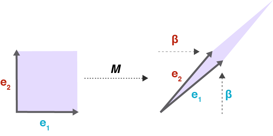
In this case, the off-diagonal elements of $M$ shear the matrix in two dimensions. The larger the value of $\beta$, provided $0 < \beta < 1$, the smaller the determinant of $M$. If $\beta \geq 1$, then $M$ is no longer positive semi-definite because the determinant is either $0$ or negative.

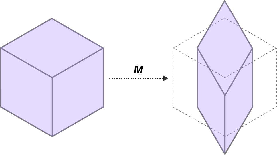
I like this geometrical intuition for the kernels of DPPs because it generalizes better in my mind. I find generalizing Equation $1$ difficult, but I can imagine a determinant of a kernel matrix in three dimensions. As the off-diagonal elements of this kernel matrix increase, the unit cube in 3D space is sheared more and more, just like in the 2D case. For example, consider again the probability of three elements from a DPP, $\mathcal{P}(x_i, x_j, x_k)$. What if $K_{jk} = K_{kj}$ was high? Then the matrix transformation represented by $K_A$ would be sheared along the $kj$-plane (Figure $3$). Since the probability of the triplet is proportional to the determinant of this matrix, the probability of the triplet decreases.

Figure 3: (Left) The unit cube in $\mathbb{R}^3$. (Right) The unit cube sheared in two dimensions. The determinant of a matrix $M$ that models this transformation is less than $1$.

Gram matrices

There’s another way to think of the geometry of the determinant in relation to a DPP. Consider a realization of $\mathcal{P}$, $X = \{x_1, x_2, \dots, x_r \}$. We can construct a $n \times n$ positive semi-definite matrix in the following way:

$K = X^{\top} X$

In this case, the determinant of $K$ is equal to the squared volume of the parallelepiped spanned by the vectors in $X$. To see this, recall two facts. First, recall that $\det(M^{\top}) = \det(M)$ for any matrix $M$. And second, note that in general, the absolute value of the determinant of real vectors is equal to the volume of the parallelepiped spanned by those vectors. Then we can write:

$\det(K) = \det(X) \det(X) = \text{vol}^2(\{X_i\}_{i=1}^{k})$

This is a useful way to think about DPPs because it means that if we construct our kernel $K$ in the manner above, we have a very nice intuition for our model: if $X$ is a realization from our point process $\mathcal{P}$ over $\mathcal{X}$, then as the points in $X$ move farther apart, the probability of sampling $X$ increases. This is because now $K$ is just a Gram matrix, i.e.:

$K = \begin{bmatrix} \langle x_1, x_1 \rangle & \langle x_1, x_2 \rangle & \dots & \langle x_1, x_r \rangle \\ \langle x_2, x_1 \rangle & \langle x_2, x_2 \rangle & \dots & \langle x_2, x_r \rangle \\ \vdots & \vdots & \ddots & \vdots \\ \langle x_r, x_1 \rangle & \langle x_r, x_2 \rangle & \dots & \langle x_r, x_r \rangle \end{bmatrix}$

and if two elements $x_i$ and $x_j$ have a larger inner product, then the probability of them co-occuring in a realization of our point process decreases. For real matrices, this inner product just the dot product, which has a simple, geometrical intuition.

Conclusion

DPPs are an interesting way to model repulsive systems. In probabilistic machine learning, they have been used as a prior for latent variable models (Zou & Adams, 2012)—think of a DPP with over a Gram matrix of latent variable parameters—, and in optimization, they have been used for diversifying mini-batches (Zhang et al., 2017), which may lead to stochastic gradients with lower variance, especially in contexts such as imbalanced data.