A Geometrical Understanding of Matrices

Beyond systems of equations

I took linear algebra in college, but the main thing I remember from the course was solving systems of linear equations by converting matrices to row echelon form. I did well in the class, but I had little intuition for matrices as geometric objects and almost none of the material stuck. In graduate school, I have discovered that having such a geometrical intuition for matrices—and for linear algebra more broadly—makes many concepts easier to understand, chunk, and remember.

For example, computing the determinant of a matrix is tedious. But if we think of the determinant of a matrix as the signed scale factor representing how much a matrix transforms the volume of an $n$-cube into an $m$-dimensional parallelepiped, it is straightforward to see why a matrix with a determinant of $0$ is singular. It is because the matrix is collapsing space along at least one dimension.

The goal of this post is to lay the ground work for understanding matrices as geometric objects. I focus on matrices because they effect how I think of vectors, vector spaces, the determinant, null spaces, spans, ranks, inverse matrices, singular values, and so on. In my mind, every one of these concepts is easier to understand with a strong, geometrical understanding of matrices. For simplicity, I will focus on real-valued matrices and vectors, and I error on the side of intuitive examples rather than generalizations.

Matrices as linear transformations

In linear algebra, we are interested in equations of the following form:

$\textbf{b} = A \textbf{x}$

Where $\textbf{b} \in \mathbb{R}^{m}$, $A \in \mathbb{R}^{m \times n}$, and $\textbf{x} \in \mathbb{R}^{n}$. One way to think about this equation is that $A$ represents a system of $m$ linear equations, each with $n$ variables, and $\textbf{x}$ represents a solution to this system. But there is another way to think of the matrix $A$, which is as a linear function $f$ from $\mathbb{R}^n$ to $\mathbb{R}^m$:

$f(\textbf{x}) = A \textbf{x}$

In my mind, the easiest way to see how matrices are linear transformations is to observe that the columns of a matrix $A$ represent where the standard basis vectors in $\mathbb{R}^n$ map to in $\mathbb{R}^m$. Let’s look at an example. Recall that the standard basis vectors in $\mathbb{R}^3$ are:

$\textbf{e}_1 = \begin{bmatrix} 1 \\ 0 \\ 0 \end{bmatrix} \qquad \textbf{e}_2 = \begin{bmatrix} 0 \\ 1 \\ 0 \end{bmatrix} \qquad \textbf{e}_3 = \begin{bmatrix} 0 \\ 0 \\ 1 \end{bmatrix}$

By definition, this means that every vector in $\mathbb{R}^3$ is a linear combination of this set of basis vectors:

$\textbf{x} = \begin{bmatrix} x_1 \\ x_2 \\ x_3 \end{bmatrix} = x_1 \begin{bmatrix} 1 \\ 0 \\ 0 \end{bmatrix} + x_2 \begin{bmatrix} 0 \\ 1 \\ 0 \end{bmatrix} + x_3 \begin{bmatrix} 0 \\ 0 \\ 1 \end{bmatrix}$

Now let’s see what happens when we matrix multiply one of these standard basis vectors, say $\textbf{e}_2$, by a transformation matrix $A$:

$\overbrace{ \vphantom{\begin{bmatrix}0\\0\\0\end{bmatrix}} \left[\begin{array}{c|c|c} 1 & \textcolor{#bc2612}{2} & 0 \\ -5 & \textcolor{#bc2612}{3} & 1 \end{array}\right] }^{A} \overbrace{ \vphantom{\begin{bmatrix}0\\0\\0\end{bmatrix}} \begin{bmatrix} 0 \\ 1 \\ 0 \end{bmatrix} }^{\textbf{e}_2} = \begin{bmatrix} 0 + \textcolor{#bc2612}{2} + 0 \\ 0 + \textcolor{#bc2612}{3} + 0 \end{bmatrix} = \begin{bmatrix} \textcolor{#bc2612}{2} \\ \textcolor{#bc2612}{3} \end{bmatrix}$

In words, the second column of $A$ tells us where the second basis vector in $\mathbb{R}^3$ maps to in $\mathbb{R}^2$. If we horizontally stack the standard basis vectors into a $3 \times 3$ matrix, we can see where each basis vector maps to in $\mathbb{R}^2$ with a single matrix multiplication:

$\left[\begin{array}{c|c|c} 1 & 2 & 0 \\ -5 & 3 & 1 \end{array}\right] \left[\begin{array}{c|c|c} \textcolor{#11accd}{1} & \textcolor{#bc2612}{0} & \textcolor{#807504}{0} \\ \textcolor{#11accd}{0} & \textcolor{#bc2612}{1} & \textcolor{#807504}{0} \\ \textcolor{#11accd}{0} & \textcolor{#bc2612}{0} & \textcolor{#807504}{1} \end{array}\right] = \left[\begin{array}{c|c|c} \textcolor{#11accd}{1} & \textcolor{#bc2612}{2} & \textcolor{#807504}{0} \\ \textcolor{#11accd}{-5} & \textcolor{#bc2612}{3} & \textcolor{#807504}{1} \end{array}\right]$

Now here’s the cool thing. We can express any transformed $2$-vector as a linear combination of $f(\textbf{e}_1)$, $f(\textbf{e}_2)$, and $f(\textbf{e}_3)$, where the coefficients are the components of the untransformed $3$-vector. For example, if $\textbf{x} = \begin{bmatrix} 1.2 & 1.5 & -2 \end{bmatrix}^{\top}$, then:

$\overbrace{ \vphantom{\begin{bmatrix}0\\0\\0\end{bmatrix}} \left[\begin{array}{c|c|c} 1 & 2 & 0 \\ -5 & 3 & 1 \end{array}\right]}^{A} \overbrace{ \vphantom{\begin{bmatrix}0\\0\\0\end{bmatrix}} \begin{bmatrix} 1.2 \\ 1.5 \\ -2 \end{bmatrix}}^{\textbf{x}} = \overbrace{ \vphantom{\begin{bmatrix}0\\0\\0\end{bmatrix}} \begin{bmatrix} 4.2 \\ -3.5 \end{bmatrix}}^{f(\textbf{x})} \tag{1}$

$1.2 \overbrace{\begin{bmatrix} 1 \\ -5 \end{bmatrix}}^{f(\textbf{e}_1)} + 1.5 \overbrace{\begin{bmatrix} 2 \\ 3 \end{bmatrix}}^{f(\textbf{e}_2)} - 2 \overbrace{\begin{bmatrix} 0 \\ 1 \end{bmatrix}}^{f(\textbf{e}_3)} = \begin{bmatrix} 1.2 + 3 + 0 \\ -6 + 4.5 - 2 \end{bmatrix} = \overbrace{\begin{bmatrix} 4.2 \\ -3.5 \end{bmatrix}}^{f(\textbf{x})} \tag{2}$

It’s worth staring at these equations for a few minutes. In my mind, seeing Equations $1$ and $2$ together helped me understand why matrix multiplication is defined as it is. When we perform matrix multiplication, we are projecting a vector or vectors into a new space defined by the columns of the transformation matrix. And $f(\textbf{x})$ is just a linear combination of the columns of $A$, where the coefficients are the components of $\textbf{x}$.

In my mind, changing how we see the equation $\textbf{b} = A \textbf{x}$ is not trivial. In the textbook Numerical Linear Algebra (Trefethen & Bau III, 1997), the authors claim that seeing matrices this way is “essential for a proper understanding of the algorithms of numerical linear algebra.”

This linearity is what allows us to say concretely that any linear transformation, $f: \mathbb{R}^n \rightarrow \mathbb{R}^m$, can be represented as a linear combination of the transformed basis vectors of $\textbf{x}$, which can be encoded as a matrix-vector multiplication:

$\begin{aligned} \textbf{x} &= x_1 \textbf{e}_1 + x_2 \textbf{e}_2 + \dots + x_n \textbf{e}_n \\ f(\textbf{x}) &= f(x_1 \textbf{e}_1 + x_2 \textbf{e}_2 + \dots + x_n \textbf{e}_n) \\ &= f(x_1 \textbf{e}_1) + f(x_2 \textbf{e}_2) + \dots + f(x_n \textbf{e}_n) && \text{Additivity} \\ &= x_1 f(\textbf{e}_1) + x_2 f(\textbf{e}_2) + \dots + x_n f(\textbf{e}_n) && \text{Homogeneity of degree $1$} \\ &= \left[\begin{array}{c|c|c|c} f(\textbf{e}_1) & f(\textbf{e}_2) & \dots & f(\textbf{e}_n) \end{array}\right] \textbf{x} \end{aligned}$

See the Appendix for a proof of the linearity of matrix transformations.

Visualizing matrix transformations

The linearity of matrix transformations can be visualized beautifully. For ease of visualization, let’s only consider $2 \times 2$ matrices, which represent linear transformations from $\mathbb{R}^2$ to $\mathbb{R}^2$. For example, consider the following matrix transformation $A$ of a vector $\textbf{x} = \begin{bmatrix} 1 & 2 \end{bmatrix}^{\top}$:

$\overbrace{\left[\begin{array}{c|c|c} \textcolor{#11accd}{2} & \textcolor{#bc2612}{-1} \\ \textcolor{#11accd}{0} & \textcolor{#bc2612}{1} \end{array}\right]}^{A} \overbrace{\begin{bmatrix} 1 \\ 2 \end{bmatrix}}^{\textbf{x}} = \overbrace{\begin{bmatrix} 0 \\ 2 \end{bmatrix}}^{f(\textbf{x})}$

We can visualize two important properties of this operation (Figure $1$). First, the columns of $A$ represent where the standard basis vectors in $\mathbb{R}^2$ land in this transformed vector space.

Figure 1. (A) A vector $\textbf{x}$ is a linear combination of the standard basis vectors. (B) The vector $f(\textbf{x})$ is a linear combination of the transformed standard basis vectors.

Second, in the new vector space, the vector $f(\textbf{x})$ is a linear combination of these transformed vectors. This is particularly useful to visualize by coloring unit squares and seeing how they are transformed. You can imagine that not just a vector is transformed by a matrix but that all of $\mathbb{R}^n$ is transformed an $m \times n$ matrix. Note that the determinant of the matrix is also visualized here. It is $2$.

Types of linear transformations

Now that we have some intuition for how matrix transformations represent linear functions, we might want to ask: what kind of transformations can we perform with matrices? A consequence of the linearity of matrix transformations is that we can only modify a vector space in particular ways such as by rotating, reflecting, scaling, shearing, and projecting. Intuitively, the hallmark of a linear transformation is that evenly spaced points before the transformation are evenly spaced after the transformation (Figure $2\text{a}$).

Figure 2: (A) Examples of linear transformations. Clockwise from top left: untransformed $\mathbb{R}^2$, scaling along the $x$-axis, rotation, projection onto $\mathbb{R}$, reflection about the $y$-axis, shear. (B) An example of a nonlinear transformation of $\mathbb{R}^2$.

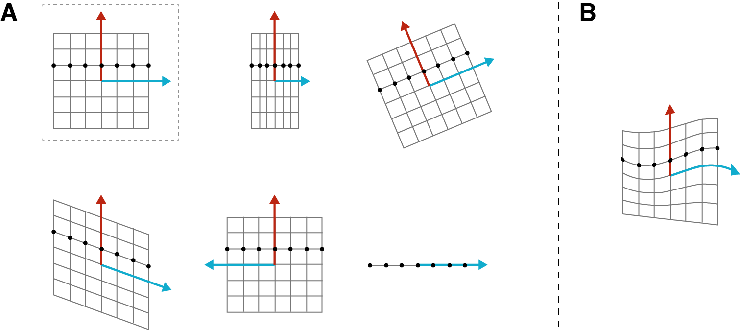
This makes sense. Linear functions are polynomials of degree one or less, meaning variables change at fixed rates. Conversely, what we cannot represent with a linear transformation is anything that would deform the space in such a way that evenly spaced points in $\mathbb{R}^n$ are unevenly spaced in $\mathbb{R}^m$ (Figure $2\text{b}$).

Now let’s look at some specific types of matrix transformations. To keep things simple, we’ll only consider square $n \times n$ matrices. This is by no means an exhaustive or formal look at every type of matrix. The idea is to see how our geometrical understanding so far relates to familiar types of matrices.

Diagonal matrices

In my opinion, a diagonal matrix is the easiest matrix to understand once you understand that the columns of a matrix $A$ represent where the standard basis vectors map to in a new vector space defined by $A$. For example, consider an arbitrary $n \times n$ diagonal matrix with scalar values $\alpha_1, \alpha_2, \dots, \alpha_n$ along its diagonal. If we think of the columns of the matrix as defining a new vector subspace, it is clear that each component in a transformed vector $\textbf{x}$ is only modified by one value on the diagonal:

$\begin{bmatrix} \textcolor{#11accd}{\alpha_1} & & & & \\ & \ddots & & & \\ & & \textcolor{#bc2612}{\alpha_i} & & \\ & & & \ddots & \\ & & & & \textcolor{#807504}{\alpha_n} \end{bmatrix} \begin{bmatrix} x_1 \\ \vdots \\ x_i \\ \vdots \\ x_n \end{bmatrix} = x_1 \begin{bmatrix} \textcolor{#11accd}{\alpha_1} \\ \phantom{\vdots} \\ \phantom{\vdots} \\ \phantom{\vdots} \\ \phantom{\vdots} \end{bmatrix} + \dots + x_i \begin{bmatrix} \phantom{\vdots} \\ \phantom{\vdots} \\ \textcolor{#bc2612}{\alpha_i} \\ \phantom{\vdots} \\ \phantom{\vdots} \end{bmatrix} + \dots + x_n \begin{bmatrix} \phantom{\vdots} \\ \phantom{\vdots} \\ \phantom{\vdots} \\ \phantom{\vdots} \\ \textcolor{#807504}{\alpha_n} \end{bmatrix}$

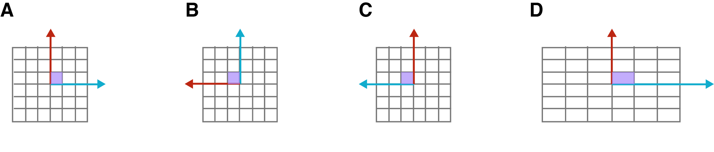
This means a diagonal matrix is constrained in how it can modify a set of vectors (Figure $3$). For example, it can stretch the $i$-th component of a vector with $\alpha_i > 1$, or it can reflect the $i$-th component with $\alpha_i < 0$. You cannot shear a vector subspace with a diagonal matrix.

Figure 3: Examples of transformations due to diagonal matrices. (A) Unit square. (B) Rotation by flipping columns. (C) Reflection by changing the sign of a column. Note that this transformation is unachievable through rotation. (D) Stretching by multiplying a column by a scalar.

Note that the identity matrix is a diagonal matrix where $\forall i, \alpha_i = 1$, meaning the standard basis vectors are not changed. It has a determinant of $1$ because it does not modify a vector subspace.

Shear matrices

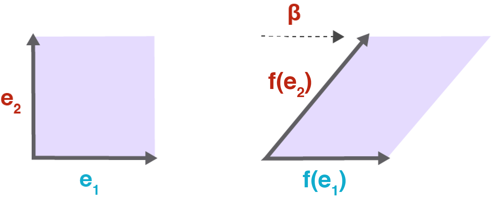
A shear matrix is so-named because you can imagine the unit square shearing. We can achieve shear with an off-diagonal element:

$\begin{bmatrix} \alpha_1 & \dots & \textcolor{#bc2612}{\beta} & & \\ & \ddots & \vdots & & \\ & & \textcolor{#bc2612}{\alpha_i} & & \\ & & & \ddots & \\ & & & & \alpha_n \end{bmatrix} \begin{bmatrix} x_1 \\ \vdots \\ x_i \\ \vdots \\ x_n \end{bmatrix} = x_1 \begin{bmatrix} \textcolor{#11accd}{\alpha_1} \\ \phantom{\vdots} \\ \phantom{\vdots} \\ \phantom{\vdots} \\ \phantom{\vdots} \end{bmatrix} + \dots + x_i \begin{bmatrix} \textcolor{#bc2612}{\beta} \\ \phantom{\vdots} \\ \textcolor{#bc2612}{\alpha_i} \\ \phantom{\vdots} \\ \phantom{\vdots} \end{bmatrix} + \dots + x_n \begin{bmatrix} \phantom{\vdots} \\ \phantom{\vdots} \\ \phantom{\vdots} \\ \phantom{\vdots} \\ \textcolor{#807504}{\alpha_n} \end{bmatrix}$

Without the off-diagonal element $\beta$, this transformation would just stretch $x_1$ by $\alpha_1$. The off-diagonal element means that a transformed vector’s $1$-st component is a linear combination of $\beta$ and $\alpha_1$. This results in a unit square that is sheared because one dimension is now a function of two dimensions (Figure $4$).

Figure 4: (Left) A unit square and (Right) the unit square sheared with an off-diagonal element $\beta$.

The matrix visualized in Figure $1$ is a concrete example of a shear matrix.

Orthogonal matrix

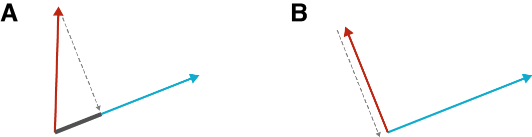
An orthogonal matrix $A$ is a square matrix whose columns and rows are orthogonal unit vectors. Let $\textbf{a}_i$ represent the $i$-th column vector of $A$. Recall that two vectors are orthogonal if the dot product between them is $0$. Geometrically, this means that if you were to project one vector onto another, it would turn into a point rather than a line (Figure $5$).

Figure 5: (A) The dot product between two vectors that are not orthogonal. The length of the gray line is the scalar result of the dot product. (B) The dot product between two orthogonal vectors is $0$ because projecting one vector onto the other results in a $0$ vector with $0$ length.

So the columns $\textbf{a}_i^{\top} \textbf{a}_j = 0$ for all $i \neq j$. And since the columns are unit vectors, then $\textbf{a}_i^{\top} \textbf{a}_i = 1$. An immediate consequence of this is that if a matrix $A \in \mathbb{R}^{n \times n}$ is orthogonal, then:

$A A^{\top} = A^{\top} A = I_n$

If this is not obvious, write out the matrices explicitly as column and row vectors:

$A^{\top} A = \left[\begin{array}{c} \textbf{a}_1^{\top} \\ \hline \textbf{a}_2^{\top} \\ \hline \vdots \\ \hline \textbf{a}_n^{\top} \end{array}\right] \left[ \begin{array}{c|c|c|c} \textbf{a}_1 & \textbf{a}_2 & \dots & \textbf{a}_n \end{array} \right] = \begin{bmatrix} 1 & & & \\ & 1 & & \\ & & \ddots & \\ & & & 1 \end{bmatrix} = I_n$

But what is the geometric intuition for orthogonal matrices? In words, an orthogonal matrix can rotate or flip a vector space, but it will not stretch it or compress it. But we can make our thinking more rigorous. The key is to observe a few key properties of orthogonal matrices:

1. Angles are preserved

Given a set of vectors, $\{\textbf{v}_1, \textbf{v}_2, \dots \textbf{v}_k \}$, which we can represent as columns in a matrix $V$, an orthogonal matrix $A$ will preserve all the angles between pairs of vectors in this set after the transformation $AV$. To see this, let $\textbf{v}_i \cdot \textbf{v}_j$ denote the dot product between vectors $\textbf{v}_i$ and $\textbf{v}_j$. Then,

$\begin{aligned} (A \textbf{v}_i)^{\top} (A \textbf{v}_j) &= \textbf{v}_i^{\top} A^{\top} A \textbf{v}_j \\ &= \textbf{v}_i^{\top} \textbf{v}_j \end{aligned}$

In words, all angles between pairs of vectors are preserved.

2. Lengths are preserved

Given our same set of vectors $V$, an orthogonal matrix $A$ will preserve all lengths of the vectors $\textbf{v} \in V$ after the transformation $AV$. This proof is just a small modification of the previous proof:

$\begin{aligned} \lVert A \textbf{v} \lVert_2^2 &= (A \textbf{v})^{\top} (A \textbf{v}) \\ &= \textbf{v}^{\top} A^{\top} A \textbf{v} \\ &= \textbf{v}^{\top} \textbf{v} \\ &= \lVert \textbf{v} \rVert_2^2 \end{aligned}$

In words, the length of any vector in $V$ is preserved after transformation.

3. Area is preserved

Note that the determinant of an orthogonal matrix is either $1$ or $-1$. This is because,

$1 = \det(I_n) = \det(A^{\top} A) = \det(A^{\top}) \det(A) = (\det(A))^2$

Since the determinant represents the signed factor that the area of an $n$-cube is multiplied by when being transformed by a matrix, a determinant of $1$ or $-1$ means the cube is only rotated or reflected.

To summarize the previous three points: angles, lengths, and areas of a vector space transformed by an orthogonal matrix are all preserved. In my mind, this is a beautiful result. We have a geometric notion of an orthogonal matrix as a function that can only rotate or reflect a vector space, but we can combine this intuition with formal mathematical ideas such as orthogonality of vectors, the definition of the dot product, and the determinant to say something that is mathematically precise.

Composing linear functions

Since $f(g(x))$ is linear if both $f$ and $g$ are linear, we can compose matrix transformations using matrix multiplications. In fact, because of singular value decomposition (SVD), we make a very strong claim: any matrix $A \in \mathbb{R}^{m \times n}$ has a singular value decomposition $U \Sigma V^{\top}$ where $U \in \mathbb{R}^{m \times m}$ and $V \in \mathbb{R}^{n \times n}$ are orthogonal matrices and $\Sigma \in \mathbb{R}^{m \times n}$ is diagonal. Intuitively, this means we can decompose any matrix transformation into simpler transformations such as unitary transformations and diagonal transformations. This falls out of the fact that the image of the unit sphere under any matrix transformation is a hyperellipse.

I want to save SVD for a future post, but let’s look at a simple example of matrix multiplication as function composition from (Paeth, 1986), who claims but does not prove that any $2 \times 2$ rotation matrix can be decomposed into three shear matrices. Following the example in that paper, consider decomposing a rotation matrix $R$ and three shear matrices $M_{i \in \{1,2,3\}}$:

$\overbrace{\begin{bmatrix} \cos(\theta) & -\sin(\theta) \\ \sin(\theta) & \cos(\theta) \end{bmatrix}}^{R} = M_3 \times M_2 \times M_1$

$M_1 = \begin{bmatrix} 1 & \alpha \\ 0 & 1 \end{bmatrix} \qquad M_2 = \begin{bmatrix} 1 & 0 \\ \beta & 1 \end{bmatrix} \qquad M_3 = \begin{bmatrix} 1 & \gamma \\ 0 & 1 \end{bmatrix}$

Using a little trigonometry, we can solve for $\alpha = -\tan(\frac{\theta}{2})$, $\beta = \sin(\theta)$, and $\gamma = -\tan(\frac{\theta}{2})$. See the Appendix for a derivation. We can sanity check our work visualizing the matrix transformations for a specific $\theta$, say $\theta = \frac{\pi}{3}$ (Figure $6$).

Figure 6: An original vector space (left) gets transformed into a rotated vector space (right) by the application of three matrix transformations.

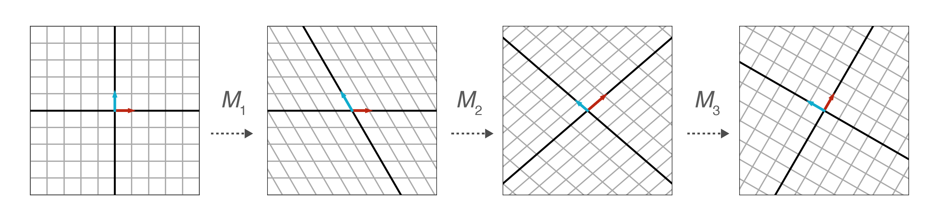
I think this is a really beautiful way to think about matrix multiplication, and it also drives home the utility of a geometrical understanding. For example, image shearing and then rotating a unit square. Now imagine applying the rotation matrix first and then shearing the rotated matrix—be sure to shear with respect to the standard basis vectors, not along an axis parallel with the rotated matrix! You won’t get the same resultant matrix. (It may help to sketch this out.) What this means that matrix multiplication is not necessarily commutative, and this is a property you can visualize rather than just remember.

Properties of matrices

With a geometrical understanding of matrices as linear transformations, many concepts in linear algebra are easier to appreciate. Here are just a concepts that are, in my mind, easier to understand geometrically.

Invertibility

Thinking of a matrix as a geometric transformation or projection, it should be clear that a rectangular matrix cannot be invertible. This is because a rectangular matrix projects vectors into either a higher- or lower-dimensional space. Imagine you found an apple lying on the ground beneath an apple tree. Can you tell me how high it was before it fell to the ground?

Rank

The rank of a matrix $A$ is the maximal number of linearly independent columns of $A$. Again, if we think of the columns of a matrix as defining where the standard basis vectors land after the transformation, then a low-rank matrix creates linear dependencies between standard basis vectors. The linear dependence between columns means that any projection will map a higher-dimensional vector space to a lower-dimensional vector space.

Null space

The null space is the set of all vectors that land on the origin or become null after a transformation. For example, if a $3 \times 3$ matrix has rank $2$, that means it projects all the points in a 3-dimensional space onto a plane. This means there are a line of vectors that all land on the origin. If this is hard to visualize, imagine flattening a cardboard box in which the origin is in the center of the box. As you flatten the box, there must a line of vectors that all collapse to the origin.

Spectral norm

The spectral norm computes the maximum singular value $\sigma_1$ of a matrix:

$\sigma_1 = \max_{\lVert \textbf{x} \rVert_2 \neq \textbf{0}} \frac{\lVert A \textbf{x} \rVert_2}{\lVert \textbf{x} \rVert_2}$

Since a matrix transforms a vector, we can think of the spectral norm as measuring the maximum amount that a matrix can “stretch” a vector. Many methods and proofs in numerical and randomized linear algebra rely on this norm. For example, algorithms in (Mahoney, 2016) use the spectral norm to bound randomized approximations of matrix multiplication.

Determinant

The determinant has the property that it is multiplicative. That is:

$\det(AB) = \det(A)\det(B)$

You can easily find formal proofs of this, but let’s convince ourselves that this is at least plausible through geometrical intuition. Consider a scenario in which $A$ and $B$ are defined as follows:

$A = \begin{bmatrix} 3 & 0 \\ 0 & 1 \end{bmatrix} \qquad B = \begin{bmatrix} 2 & 0 \\ 0 & 1 \end{bmatrix}$

Our geometrical understanding of matrices suggests that matrix $A$ dilates $\textbf{e}_1$ by $3$ and matrix $B$ dilates $\textbf{e}_1$ by $2$. Can you see why the determiant is multiplicative (Figure $7$)?

Figure 7: (Left) The unit square in $\mathbb{R}^2$. (Middle) The unit square transformed by matrix $A$. (Right) The unit square transformed by matrix $AB$.

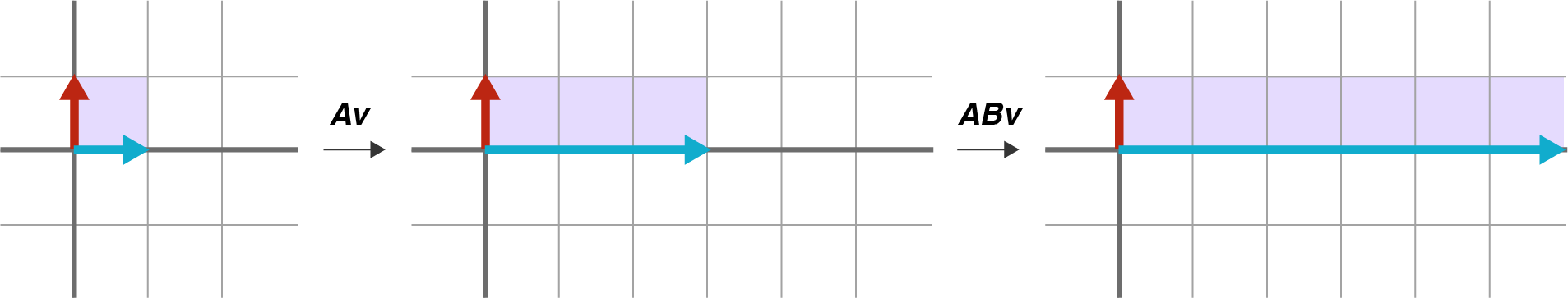
The determinant of $A$ is $3$, while the determinant of $B$ is $2$. And what is the determinant of $AB$? It is $6$ because it dilates a unit cube by $6$.

Another cool property of the determinant that is easy to visualize is its sign. The sign of the determinant is positive if the matrix does not change the chirality of the space and negative if it does. This is, I think, easy to visualize (Figure $8$).

Figure 8: (Left) A right hand, palm facing the screen, on a unit square. (Right) The chirality of the right hand has been changed by a matrix transformation with determinant $-1$.

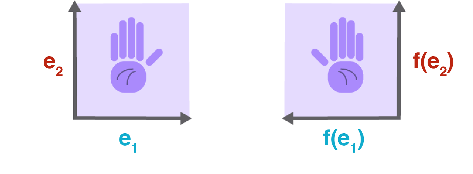
Imagine a chiral object—that is, an object that cannot be mapped to its mirror image by rotations and translations alone, for example a hand. A matrix transformation on that chiral object that changes its chirality changes the sign of the determinant.

Conclusion

While thinking about these ideas, I came across this lecture by Amritanshu Prasad, who argues at the end of the video for a geometrical understanding:

Most of us think fairly geometrically to start with, and algebra comes as part of training. Also, a lot of mathematics comes from trying to model problems in physics where we really need to think geometrically. So in that sense, a definition that is geometric has much more relationship to the physical world around us and also perhaps gives us a better intuition about the object we’re studying.

Mathematics is a contact sport, and I have no illusions that a geometrical understanding that is not paired with rigorous, numerical understanding is sufficient. It is impossible to deeply understand a mathematical idea if you cannot formalize it. That said, I have found that my ability to “think in linear algebra” has been strengthened by a better geometrical understanding of the material.

Acknowledgements

I thank Philippe Eenens for helpful suggestions for clarifying the notation.

Appendix

1. Proof that matrices are linear transformations

To prove that a function $f$ is linear, we need to show two properties:

1. $f(a) + f(b) = f(a + b)$
2. $f(ca) = c f(a)$

Let $A$ be an $m \times n$ vector, so the $i$-th column in $A$, $\textbf{a}_i$, is an $m$-vector and there are $n$ such vectors. And let $\textbf{v}$ and $\textbf{u}$ be two $n$-vectors. Then we can express a function $f$ as the linear combination of the columns of $A$ where the coefficients in are the scalar components in $\textbf{v}$ and $\textbf{u}$:

$\begin{aligned} f(\textbf{v}) &= A \textbf{v} = v_1 \textbf{a}_1 + v_2 \textbf{a}_2 + \dots + v_n \textbf{a}_n \\ f(\textbf{u}) &= A \textbf{u} = u_1 \textbf{a}_1 + u_2 \textbf{a}_2 + \dots + u_n \textbf{a}_n \end{aligned}$

Proving both properties is straightforward with this representation because we only need to rely on properties of scalar addition and multiplication.

Property 1

$\begin{aligned} f(\textbf{u}) + f(\textbf{v}) &= A \textbf{u} + A \textbf{v} \\ &= u_1 \textbf{a}_1 + u_2 \textbf{a}_2 + \dots + u_n \textbf{a}_n + v_1 \textbf{a}_1 + v_2 \textbf{a}_2 + \dots + v_n \textbf{a}_n \\ &= (u_1 + v_1) \textbf{a}_1 + (u_2 + v_2) \textbf{a}_2 + \dots + (u_n + v_n) \textbf{a}_n \\ &= A(\textbf{u} + \textbf{v}) \\ &= f(\textbf{u} + \textbf{v}) \end{aligned}$

Property 2

$\begin{aligned} f(c\textbf{u}) &= A(c \textbf{u}) \\ &= c u_1 \textbf{a}_1 + c u_2 \textbf{a}_2 + \dots + c u_n \textbf{a}_n \\ &= c(u_1 \textbf{a}_1 + u_2 \textbf{a}_2 + \dots + u_n \textbf{a}_n) \\ &= c A(\textbf{u}) \\ &= c f(\textbf{u}) \end{aligned}$

2. Derivation for rotation matrix decomposition

To solve for $\alpha$, $\beta$, and $\gamma$ in terms of $\theta$, let’s first multiply our matrices:

$\overbrace{\begin{bmatrix} 1 & \alpha \\ 0 & 1 \end{bmatrix} \begin{bmatrix} 1 & 0 \\ \beta & 1 \end{bmatrix}}^{M_1 \times M_2} = \begin{bmatrix} 1 + \alpha \beta & \alpha \\ \beta & 1 \end{bmatrix}$

$\overbrace{\begin{bmatrix} 1 + \alpha \beta & \alpha \\ \beta & 1 \end{bmatrix} \begin{bmatrix} 1 & \gamma \\ 0 & 1 \end{bmatrix}}^{M_1 \times M_2 \times M_3} = \begin{bmatrix} 1 + \alpha \beta & \gamma + \alpha \beta \gamma + \alpha \\ \beta & \beta \gamma + 1 \end{bmatrix}$

We are given that a $2 \times 2$ rotation matrix is equivalent to these three shear matrices:

$\begin{bmatrix} \cos(\theta) & - \sin(\theta) \\ \sin(\theta) & \cos(\theta) \end{bmatrix} = \begin{bmatrix} 1 + \alpha \beta & \gamma + \alpha \beta \gamma + \alpha \\ \beta & \beta \gamma + 1 \end{bmatrix}$

Now let’s solve. Immediately, we have:

$\beta = \sin(\theta)$

We can use this to solve for $\alpha$:

$\begin{aligned} \cos(\theta) &= 1 + \alpha \beta \\ &= 1 + \alpha \sin(\theta) \\ \alpha &= \frac{\cos(\theta) - 1}{\sin(\theta)} \\ &= -\frac{1 - \cos(\theta)}{\sin(\theta)} \\ &= - \tan\Big(\frac{\theta}{2}\Big) \end{aligned}$

Finally, let’s solve for $\gamma$:

$\begin{aligned} \cos(\theta) &= \beta \gamma + 1 \\ &= \sin(\theta) \gamma + 1 \\ \frac{\cos(\theta) - 1}{\sin(\theta)} &= \gamma \\ \gamma &= - \frac{1 - \cos(\theta)}{\sin(\theta)} \\ &= - \tan\Big(\frac{\theta}{2}\Big) \end{aligned}$