Why Metropolis–Hastings Works

Metropolis–Hastings (MH) is an elegant algorithm that is based on a truly deep idea. Suppose we want to sample from a target distribution $\pi^*$. We can evaluate $\pi^*$, just not sample from it. MH performs a random walk according to a Markov chain whose stationary distribution is $\pi^*$. At each step in the chain, a new state is proposed and either accepted or rejected according to a dynamically calculated probability, called the acceptance criteria. The Markov chain is never explicitly constructed; we cannot save the transition probability matrix to disk or print one of its rows. However, if the MH algorithm is run for long enough—until the Markov chain mixes—, then the probability of being on a given state in the chain is equal to the probability of the associated sample. Thus, walking the Markov chain and recording states is, in the long-run, like sampling from $\pi^*$.

This should be mind-blowing. This is not obvious. If these ideas are new, you should have to read the above paragraph twice. However, my go-to authors for excellent explanations of machine learning ideas—(Bishop, 2006; MacKay, 2003; Murphy, 2012)—as well as most blogs introduce MH by presenting just the algorithm’s acceptance criteria with no justification for why the algorithm works. For example, after MacKay introduces notation and the acceptance criteria, he writes

It can be shown that for any positive $Q$ (that is, any $Q$ such that $Q(x, x^{\prime}) > 0$ for all $x, x^{\prime}$) as $t \rightarrow \infty$, the probability distribution of $x(t)$ tends to $P(x)$.

Above, $P$ is the target distribution (what I call $\pi^{*}$), $Q$ is the proposal distribution which proposes new samples, and $x(t)$ is the sample at step $t$. That said, the above explanation completely elides the mind-blowing part: how is walking an implicit Markov chain the same as sampling from a target distribution, and how does the acceptance criteria ensure we’re randomly walking according to the desired chain?

The goal of this post is to formally justify the algorithm. The notation and proof is based on (Chib & Greenberg, 1995). I assume the reader understands Markov chains. Please see my previous post for an introduction if needed.

Notation

Consider a Markov chain with transition kernel $P(x, A)$ where $x \in \mathbb{R}^d$ and $A$ is a subset of our sample space (technically, $A \in \mathcal{B}$ where $\mathcal{B}$ is the Borel $\sigma$-field on $\mathbb{R}^d$). So in words, $P(x, A)$ is a conditional distribution function of moving from $x$ to a point in the set $A$. Note that a transition kernel is the generalization of a transition matrix in finite state-spaces. Naturally, $P(x, \mathbb{R}^d) = 1$ and self-loops are allowed, meaning that $P(x, \\{x\\})$ is not necessarily zero.

The stationary distribution of a Markov chain is defined as $\pi^{*}$ where

$\pi^{*}(\text{d}y) = \pi(y)\text{d}y = \int_{\mathbb{R}^d} P(x, \text{d}y) \pi(x) \text{d}x.$

This is just the continuous state-space analog of the discrete case. In a discrete Markov chain $\\{X_n\\}$ taking values in $D$, if the transition matrix is $\mathbf{P} = (p_{ij})\_{i,j \in D}$, then stationary distribution is

$\boldsymbol{\pi}^{*} = \boldsymbol{\pi}^{*} \mathbf{P}$

where $\boldsymbol{\pi}^{*}$ is a $D$-dimensional row vector. In words, the Markov chain has mixed when the probability of being on a given state no longer changes as we walk the chain.

The $n$-th iterate or $n$th application of the transition kernel is given by

$\begin{aligned} P^{(1)}(x, A) &= P(x, A) \\ P^{(n)}(x, A) &= \int_{\mathbb{R}^d} P^{(n-1)} (x, \text{d}y) P(y, A). \end{aligned}$

As $n$ goes to infinity, the $n$-th iterate converges to the stationary distribution or

$\pi^{*}(A) = \lim_{n \rightarrow \infty} P^{(n)}(x, A).$

The above is an alternative definition of $\pi^{*}$.

Implicit Markov chain construction

Markov chain Monte Carlo (MCMC) approaches the problem of sampling in a beautiful but nonobvious way. We want to sample from a $\pi^{*}$. Let’s imagine that $\pi^{*}$ is the stationary distribution of a particular Markov chain. If we could randomly walk that Markov chain, then we could sample from $\pi^{*}$ eventually. Thus, we need to construct a transition kernel $P(x, A)$ which converges to $\pi^{*}$ in the limit.

Suppose we represent the transition kernel as

$P(x, \text{d}y) = p(x, y) \mathbf{1}(x \notin \text{d}y) \text{d}y + r(x) \mathbf{1}(x \in \text{d}y) \tag{1}$

where $p(x, y)$ is some function, $\mathbf{1}(c)$ is an indicator random variable taking the value one if condition $c$ is true and zero otherwise, and $r(x)$ is defined as

$r(x) = 1 - \int_{\mathbb{R}^d} p(x, y) \text{d}y.$

Alternatively, we can write the kernel as

$P(x, \text{d}y) = \begin{cases} 1 - \int_{\mathbb{R}^d} p(x, y) \text{d}y & \text{if $x \in \text{d}y$} \\ p(x, y) \text{d}y & \text{else}. \end{cases}$

Thus, $r(x)$ is the probability that the Markov chain remains at $x$, and $\int_{\mathbb{R}^d} p(x, y) \text{d}y$ is not necessarily one because $r(x)$ is not necessarily zero.

Now consider the following reversibility constraint,

$\pi(x) p(x, y) = \pi(y) p(y, x). \tag{2}$

If $p(x, y)$ adheres to this constraint, then $\pi(\cdot)$ is the stationary distribution of $P(x, \cdot)$. To see this, consider the following derivation:

$\begin{aligned} \int_{\mathbb{R}^d} P(x, A) \pi(x) \text{d}x &= \int_{\mathbb{R}^d} \Big[\int_A p(x, y) \mathbf{1}(x \notin \text{d}y) \text{d}y + r(x) \mathbf{1}(x \in \text{d}y) \Big] \pi(x) \text{d}x \\ &= \int_{\mathbb{R}^d} \Big[\int_A p(x, y) \mathbf{1}(x \notin \text{d}y) \text{d}y \Big] \pi(x) \text{d}x + \int_{\mathbb{R}^d} r(x) \mathbf{1}(x \in A) \pi(x) \text{d}x \\ &= \int_{\mathbb{R}^d} \Big[\int_A p(x, y) \mathbf{1}(x \notin \text{d}y) \text{d}y \Big] \pi(x) \text{d}x + \int_A r(x) \pi(x) \text{d}x \\ &= \int_A \Big[\int_{\mathbb{R}^d} p(x, y) \pi(x) \text{d}x \Big] \mathbf{1}(x \notin \text{d}y)\text{d}y + \int_A r(x) \pi(x) \text{d}x \\ &\stackrel{\star}{=} \int_A \Big[\int_{\mathbb{R}^d} p(y, x) \pi(y) \text{d}x \Big] \mathbf{1}(x \notin \text{d}y)\text{d}y + \int_A r(x) \pi(x) \text{d}x \\ &= \int_A (1 - r(y)) \pi(y) \text{d}y + \int_A r(x) \pi(x) \text{d}x \\ &= \int_A \pi(x) \text{d}x. \end{aligned}$

Step $\star$ is the key step. It only holds because of the reversibility constraint, and it’s what allows us to cancel all terms except $\pi(y) \text{d}y$.

Let’s review. We want to sample from some target distribution $\pi^{*}$. We imagine that this distribution is the stationary distribution of some Markov chain, but we don’t know the chain’s transition kernel $P(x, A)$. The above derivation demonstrates that if we define $P(x, A)$ as Equation $1$ and ensure that $p(x, y)$ adheres to the reversibility constraint in Equation $2$, then we will have found the transition kernel for a chain whose stationary distribution is our target distribution. This is the essence of Metropolis–Hastings. As we will see, MH’s acceptance criteria is constructed to ensure that the reversibility constraint is met.

Metropolis–Hastings

We want to construct the function $p(x, y)$ such that it is reversible. Consider a candidate generating density, $q(y \mid x)$. This density, as in rejection sampling, generates candidate samples $y$ conditioned on $x$ that will be either rejected or accepted depending on some criteria. Note that if $x$ and $y$ are states, this is a Markov process because no past states are considered. The future only depends on the present. Since $q(\cdot)$ is a density, $\int q(y \mid x) \text{d}y = 1$. If the following were true,

$q(y \mid x) \pi(x) = q(x \mid y) \pi(y)$

then we’re done. We’ve satisfied Equation $2$. But most likely this is not the case. For example, we might find that

$q(y \mid x) \pi(x) \geq q(x \mid y) \pi(y).$

Our random process moves from $x$ to $y$ more often than from $y$ to $x$. MH ensures equilibrium (reversibility) this by restricting some moves (samples) according to an acceptance criterion, $\alpha(x, y) \leq 1$. Thus, if a move is not made, the process returns to $x$. Intuitively, this is what allows us to balance $q(y \mid x)\pi(x)$ with $q(x \mid y)\pi(y)$. Let’s assume that moves from $x$ to $y$ happen more often than the reverse. Then our criteria would be

$\begin{aligned} q(y \mid x) \pi(x) \alpha(x, y) &= q(x \mid y) \pi(y) \\ \alpha(x, y) &= \frac{q(x \mid y) \pi(y)}{q(y \mid x) \pi(x)}. \end{aligned}$

Of course, the probabilities could be reversed, but we can handle both cases this with a single expression:

$\alpha(x, y) = \min \Bigg\{ 1, \frac{q(x \mid y) \pi(y) }{q(y \mid x) \pi(x)} \Bigg\}. \tag{3}$

If MH moves from $x$ to $y$ more than the reverse, then the numerator is greater than the denominator, and the probability of accepting a move to $y$ from $x$ goes down. If we move from $y$ to $x$ more than the reverse, the sample (move from $x$ to $y$) is accepted with probability one.

We have found our function $p(x, y)$. It is

$p_{\texttt{MH}}(x, y) = \alpha(x, y) q(y \mid x), \qquad x \neq y.$

And while it is unnecessary to write down, for completeness the full transition kernel $P_{\texttt{MH}}(x, y)$ is

$P_{\texttt{MH}}(x, y) = \overbrace{\phantom{\Bigg|} \alpha(x, y) q(y \mid x) }^{\text{prob. leaving $x$}} + \overbrace{\phantom{\Bigg|} \Big[ 1 - \int_{\mathbb{R}^d} \alpha(x, y) q(y \mid x) \text{d}y \Big] \mathbf{1}(x \in \text{d}y). }^{\text{prob. staying on $x$}}$

In summary, if we conditionally sample according to the density $q(y \mid x)$ and accept the proposed sample according to $\alpha(x, y)$, then we’ll be randomly walking according to a Markov chain whose stationary distribution is $\pi^{*}$.

Metropolis

Notice that for a symmetric conditional distribution—so $q(y \mid x) = q(x \mid y)$—, Equation $3$ simplifies to

$\alpha(x, y) = \min \Bigg\{ 1, \frac{\pi(y) }{\pi(x)} \Bigg\}.$

This is the predecessor to Metropolis–Hastings, the Metropolis algorithm invented by Nicholas Metropolis et al in 1953 (Metropolis et al., 1953). In 1970, Wilfred Hastings extended Equation $4$ to the more general asymmetrical case in Equation $3$ (Hastings, 1970). For example, if we assume that $q(y \mid x)$ is a conditional Gaussian distribution, then running the Metropolis–Hastings algorithm is equivalent to running the Metropolis algorithm.

Example: Rosenbrock density

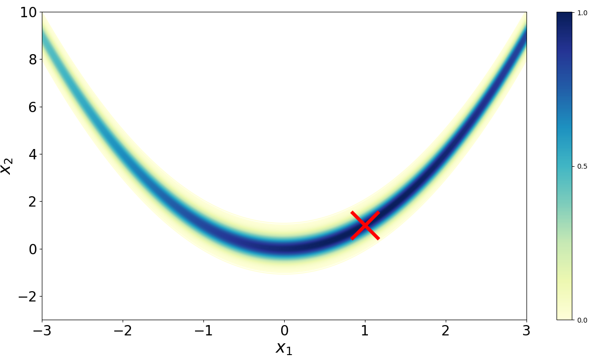
Imagine we want to sample from the Rosenbrock density (Figure $1$),

$\pi^{*}(x_1, x_2; a, b) \propto \exp\Big\{-\frac{(a - x_1)^2 + b(x_2 - x_1^2)^2}{20}\Big\}. \tag{4}$

The Rosenbrock function (Rosenbrock, 1960) is a well-known test function in optimization because while finding a minimum is relatively easy, finding the global minimum at ($1$, $1$) is less trivial. (Goodman & Weare, 2010) adapted the function to serve as a benchmark for MCMC algorithms.

Figure 1. The Rosenbrock density (Equation $4$) with $a = 1$ and $b = 100$. Darker colors indicate higher probability. The global minimum is at $(x, y) = (a, a^2) = (1, 1)$ and denoted with a red "X".

We must provide a candidate transition kernel $q(y \mid x)$. The only requirement is that we can sample conditionally from it and that $\int q(y \mid x) \text{d}y = 1$ for all $x$. Perhaps the simplest possible kernel is to simply add Gaussian noise to $x$. Thus, our candidate distribution is

$y \mid x \sim \mathcal{N}(x; 0, \sigma^2), \qquad y = x + \mathcal{N}(0, \sigma^2)$

where the variance $\sigma^2$ controls how big each step is. Since the density is symmetric, we can implement the simpler Metropolis algorithm. We can accept a proposal sample with probability $\alpha(x, y)$ by drawing a uniform random variable with support $[0, 1]$, and checking if it is less than the acceptance criteria. For our setup, we have:

import numpy as np
from   numpy.random import multivariate_normal as mvn
import matplotlib.pyplot as plt

n_iters    = 1000
samples    = np.empty((n_iters, 2))
samples[0] = np.random.uniform(low=[-3, -3], high=[3, 10], size=2)
rosen      = lambda x, y: np.exp(-((1 - x)**2 + 100*(y - x**2)**2) / 20)

for i in range(1, n_iters):
    curr  = samples[i-1]
    prop  = curr + mvn(np.zeros(2), np.eye(2) * 0.1)
    alpha = rosen(*prop) / rosen(*curr)
    if np.random.uniform() < alpha:
        curr = prop
    samples[i] = curr

plt.plot(samples[:, 0], samples[:, 1])
plt.show()

That’s it. Despite its conceptual depth, Metropolis–Hastings is surprisingly simple to implement, and it is not hard to imagine writing a more general implementation that handles Equation $3$ for any arbitrary $\pi$ and $q(\cdot)$.

Figure 2. Three randomly initialized Markov chains run on the Rosenbrock density (Equation $4$) using the Metropolis–Hastings algorithm. After mixing, each chain walks regions in regions where the probability is high. The global minimum is at $(x, y) = (a, a^2) = (1, 1)$ and denoted with a black "X".

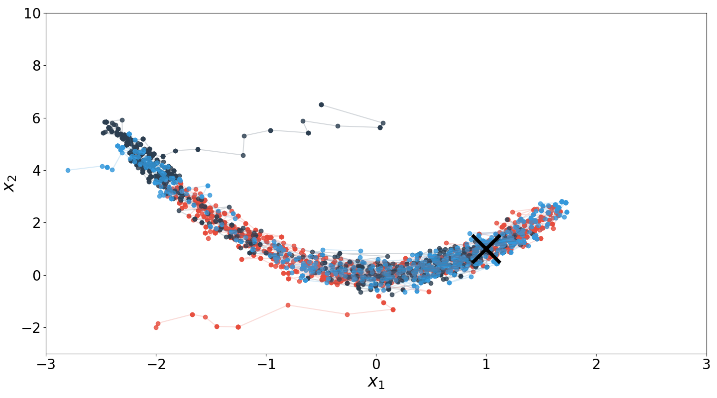
The above code is the basis for Figure $2$, which runs three Markov chains from randomly initialized starting points. This example highlights two important implementation details for Metropolis–Hastings. First, step size (or $\sigma^2$ for our candidate distribution) is important. If the step size were too large relative to the support of the Rosenbrock density, it would be difficult to sample near the distribution’s mode. Second, a so-called burn-in period in which initial samples are discarded is typically used. This is because samples before the chain starts to mix are not representative of the underlying distribution.

Conclusion

Metropolis–Hastings is a beautifully simple algorithm based on a truly original idea. We have these mathematical objects called Markov chains that, when ergodic, converge to their respective stationary distirbutions. We turn this idea on its head, and imagine that our target distribution is the stationary distribution for a given chain, and then implicitly construct that chain on the fly. The acceptance criteria ensures that the transition kernel will, in the long-run, induce the stationary distribution. Despite the algorithm being based on many deep ideas—think about how much intellectual machinery is embedded in this single paragraph—implementing the algorithm takes fewer than a dozen lines of code.

Acknowledgements

I thank Wei Deng for catching a couple typos around step $\star$.