Sampling: Two Basic Algorithms

Introduction

In probabilistic machine learning, exact inference is often difficult or impossible when we cannot sample from or estimate the properties of a particular distribution. While we can leverage conjugacy to keep the distributions tractable or use variational inference to deterministically approximate a density, we can also use randomized methods for inference using numerical sampling, sometimes called Monte Carlo methods.

While we are sometimes interested in a posterior distribution per se, we are often only interested in properties of the distribution. For example, we need the first moment of a random variable for expectation–maximization. Thus, for many problems it is sufficient to either sample from or compute moments of a distribution of interest. I will introduce sampling in the context of two basic algorithms for these tasks.

I use bold and normal letters to indicate random variables and realizations respectively. So $\mathbf{x}$ is a random variable, while $x$ is a realization of $\mathbf{x}$. I denote distributions with letters such as $p(\cdot)$, $g(\cdot)$, and so on. Thus, $p(\mathbf{x})$ refers to the distribution of $\mathbf{x}$, while $p(x)$ is the probability of $x$ under $p(\mathbf{x})$. Clearly we can evaluate $p(z)$ for a realization from another random variable $\mathbf{z} \sim q(\mathbf{z})$.

Rejection sampling

Consider the scenario in which we can evalute a density $p(\mathbf{x})$, but it is not clear how to sample from it. This may not be as abstract as it sounds. For example, consider the PDF of the exponential distribution with parameter $\lambda$,

$p(x) = \lambda e^{-\lambda x}.$

While we have a functional form for the distribution and can even prove that it satisfies some basic properties, e.g. it integrates to $1$, it may not be obvious how to sample from $p(\mathbf{x})$. What if you did not have access to scipy.stats.expon on your computer?

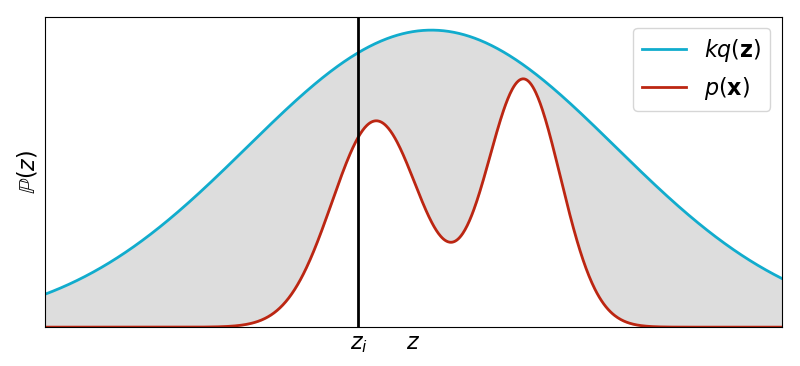
Rejection sampling works by using a proposal distribution $q(\mathbf{z})$ that we can sample from. The only constraint is that for some constant $k$,

$k q(z) \geq p(z), \quad \forall z. \tag{1}$

In words, the area under the density curve for $k q(z)$ must be greater or equal to the area under the density curve for $p(z)$ (Figure $1$).

Figure 1. Diagram of rejection sampling. The density $q(\mathbf{z})$ must be always greater than $p(\mathbf{x})$. A new sample is rejected if it falls in the gray region and accepted otherwise. These accepted samples are distributed according to $p(\mathbf{x})$. This is achieved by sampling $z_i$ from $q(\mathbf{z})$, and then sampling uniformly from $[0, k q(z_i)]$. Samples under the curve $p(z_i)$ are accepted.

The algorithm for rejection sampling is,

1. Sample $z\_i$ from $q(\mathbf{z})$.
2. Sample $u_i$ from $\text{Uniform}(0, k q(z_i))$.
3. If $u_i > p(z_i)$, reject $z_i$. Otherwise, accept it.

Why does this work? In words, the pair $(z\_i, u\_i)$ is uniformly distributed over the area under the curve of $k q(\mathbf{z})$ and since we reject samples outside of the area under the curve of $p(\mathbf{x})$, our accepted samples are uniformly distributed over the area under $p(\mathbf{x})$. While this makes some intuitive sense, I do not find such explanations particularly convincing. Let’s prove this works formally.

Proof

Let $\mathbf{x}$ and $\mathbf{z}$ be random variables with densities $p(\mathbf{x})$ and $q(\mathbf{z})$. We assume can sample from $q(\mathbf{z})$. Let $\mathbf{a}$ be a new random variable such that

$\mathbf{a} \mid z \sim \text{Bernoulli}\left(\frac{p(z)}{k q(z)}\right)$

This random variable represents the event that a sample is accepted; its conditional probability distribution is Bernoulli with a “success” parameter $p(z) / k q(z)$. We want to show that for any event $\mathcal{S}$, $\mathbb{P}(\mathbf{z} \in \mathcal{S} \mid a = 1) = \mathbb{P}(\mathbf{x} \in \mathcal{S})$. In words, we want to show that the conditional probability of an event given that we accept a realization from $q(\mathbf{z})$ is equal to the probability of that same event under $p(\mathbf{x})$. Using Bayes’ formula, we have

$\mathbb{P}(\mathbf{z} \in \mathcal{S} \mid \mathbf{a} = 1) = \frac{\mathbb{P}(\mathbf{a} = 1 \mid \mathbf{z} \in \mathcal{S}) \mathbb{P}(\mathbf{z} \in \mathcal{S})}{\mathbb{P}(\mathbf{a} = 1)}.$

Let $h(\cdot)$ denote the conditional density of $\mathbf{a}$ given $y$. Then the numerator is

$\begin{aligned} \mathbb{P}(\mathbf{a} = 1 \mid \mathbf{z} \in \mathcal{S}) \mathbb{P}(\mathbf{z} \in \mathcal{S}) &= \int_{\mathcal{S}} h(\mathbf{a} = 1 \mid z) q(z) \text{d}z \\ &= \int_{\mathcal{S}} \frac{p(z)}{k q(z)} q(z) \text{d}z \\ &= \frac{1}{k}\int_{\mathcal{S}} p(z) \text{d}z \\ &= \frac{\mathbb{P}(\mathbf{x} \in \mathcal{S})}{k}. \end{aligned}$

For the denominator, we compute the marginal of $\mathbf{a}$ by integrating out $\mathbf{z}$, giving us

$\begin{aligned} \mathbb{P}(\mathbf{a} = 1) &= \int_{\mathcal{Z}} h(\mathbf{a} = 1 \mid z) q(z) \text{d}z \\ &= \int_{\mathcal{Z}} \frac{p(z)}{k q(z)} q(z) \text{d}z \\ &= \frac{1}{k} \int_{\mathcal{Z}} p(z) \text{d}z \\ &= \frac{1}{k}. \end{aligned}$

Putting everything together, we get

$\begin{aligned} \mathbb{P}(\mathbf{z} \in \mathcal{S} \mid \mathbf{a} = 1) &= \frac{\mathbb{P}(\mathbf{x} \in \mathcal{S}) / k}{1 / k} \\ &= \mathbb{P}(\mathbf{x} \in \mathcal{S}) \end{aligned}$

as desired.

Example

Consider the task of sampling from a bimodal distribution $p(\mathbf{x})$. We can use rejection sampling with a standard Gaussian scaled by an appropriate $k$ such that Equation $1$ holds (Figure $2$).

Figure 2. Rejection sampling from a bimodal distribution (blue dots) using a Gaussian proposal distribution (red dots). Since we are uniformly sampling from our proposal distribution and rejecting any that are not in our target distribution, we reject roughly the same proportion of samples regardless of the number of samples.

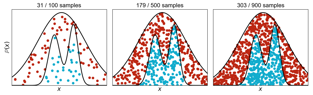
This highlights the main challenge of rejection sampling, which is computational efficiency. In this small example, we must discard roughly two-thirds of the samples in order to sample from $p(\mathbf{x})$, where $\mathbf{x}$ is a univariate random variable. If $\mathbf{x}$ were high-dimensional, we would throw out exponentially more samples.

Importance sampling

Importance sampling is a Monte Carlo method for approximating integrals. The word “sampling” is a bit confusing since, unlike rejection sampling, the method does not approximate samples from a desired distribution $p(\mathbf{x})$. In fact, we do not even have to be able to sample from $p(\mathbf{x})$.

The intuition is that a well-defined integral,

$\mathcal{I} = \int_{\mathcal{Z}} h(z) \text{d}z$

can be viewed as an expectation for a probability distribution,

$\mathbb{E}_{q}[H(\mathbf{z})] = \int_{\mathcal{Z}} H(z) q(z) \text{d}z$

where $H(\cdot)$ is

$H(z) = \frac{h(z)}{q(z)}.$

Provided $q(z) > 0$ when $h(z) \neq 0$, then $\mathcal{I} = \mathbb{E}_{q}[H(\mathbf{z})]$. Provided we can evaluate $H(z)$, we can approximate our integral using the Law of Large Numbers. We sample $N$ i.i.d. samples from the density $q(\mathbf{z})$ and then compute

$\hat{\mathcal{I}} = \frac{1}{N} \sum_{n=1}^{N} H(z_n).$

This estimator $\hat{\mathcal{I}}$ is unbiased and converges to $\mathcal{I}$ in the limit of $N$.

Now that we understand the main idea, let $p(\mathbf{x})$ be a density that we cannot sample from but that we can evaluate. Provided $\{z_n\}_{n=1}^{N}$ are i.i.d. samples from $q(\mathbf{z})$, then for a function $f$,

$\begin{aligned} \mathbb{E}_p[f(\mathbf{x})] &= \int_{\mathcal{X}} f(x) p(x) \text{d}x \\ &= \int_{\mathcal{X}} H(x) q(x) \text{d}x \\ &\approx \frac{1}{N} \sum_{n=1}^{N} H(z_n) \\ &\approx \frac{1}{N} \sum_{n=1}^{N} f(z_n) \frac{p(z_n)}{q(z_n)} \tag{2} \end{aligned}$

where $H(\cdot)$ is defined as

$H(z) = f(z) \frac{p(z)}{q(z)}.$

Thus, provided we can sample from $q(\mathbf{z})$ and evaluate $p(z)$ and $f(z)$, we can get an unbiased estimator of the expectation $\mathbb{E}_p[f(\mathbf{x})]$.

The terms $p(z_n) / q(z_n)$ in Equation $2$ are called the importance weights because for each sample, they correct the bias induced by sampling from the wrong distribution, $q(\mathbf{z})$ instead of $p(\mathbf{x})$.

There are some additional technical details, for example if we do not know the normalizing constants of $p(\mathbf{x})$ or $q(\mathbf{z})$, but the goal of this post is to provide a high-level understanding. Please consult a standard textbook for these details.

Example

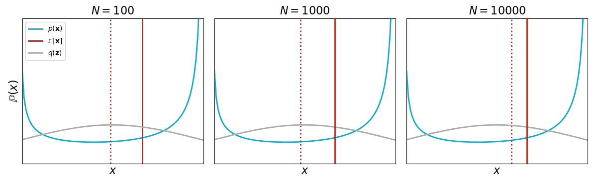
Let $\mathbf{x}$ be a continuous random variable that we know to be beta distributed with specific parameters $\alpha$ and $\beta$. (Really, we just need to be able to evaluate $p(x)$.) Imagine that we did not know this random variable’s moments. We can use importance sampling to estimate them. Recall that a continuous random variable’s expectation is

$\mathbb{E}_p[\mathbf{x}] = \int x p(x) \text{d}x$

Then if we set $f(x) = x$, we can use importance sampling to approximate the mean. We sample $N$ i.i.d. samples from $q(\mathbf{z})$ and then estimate the first moment as

$\mathbb{E}_p[\mathbf{x}] \approx \sum_{n=1}^{N} H(z_n), \quad H(z) = \frac{p(z)}{q(z)}$

Let’s draw $N$ i.i.d. samples from a Gaussian distribution, and then use the importance weights to correct the bias of drawing from the wrong distribution. As with rejection sampling, our estimate of $\mathbb{E}\_p[\mathbf{x}]$ improves as $N$ increases (Figure $3$).

Figure 3. Estimating the mean of a beta distribution with parameters $\alpha = 0.5$ and $\beta = 0.25$ (blue line) using a Gaussian distribution (gray line). As the number of samples $N$ increases, the approximation (red dashed line) of the actual mean (red solid line) improves.

Conclusion

Numerical sampling is used widely in machine learning, and the goal of this post was to give a small flavor for how these methods work. In future posts, I hope to cover more advanced methods such as Metropolis–Hastings and Gibbs Sampling.