Conjugacy in Bayesian Inference

In Bayesian inference, a prior $p(\theta)$ is conjugate to the likelihood function $p(x \mid \theta)$ when the posterior has the same functional form as the prior. This means that the two boxed terms in Bayes’ formula below have the same functional form:

$\boxed{p(\theta \mid x)} = \frac{p(x \mid \theta) \, \boxed{p(\theta)}}{\int p(x \mid \theta') p(\theta') \text{d} \theta'}$

The goal of this post is to work through an example of a conjugate prior to better understand why conjugacy is a useful property.

As a running example, imagine that we have a coin with an unknown bias. Estimating the bias $\mu$ is statistical inference; Bayesian inference is assuming a prior on $\mu$; and conjugacy is assuming the prior is conjugate to the likelihood. We will explore these ideas in order.

Modeling a Bernoulli process

We want to estimate the bias $\mu$ of our coin. First, we flip the coin $n$ times. The outcome of the $i$th coin toss is $x_i$, a Bernoulli random variable that takes values $0$ or $1$ with probability $\mu$ or $(1 - \mu)$ respectively. Without loss of generality, $1$ is a success (heads) and $0$ is a failure (tails). The sequence of coin flips is a Bernoulli process of i.i.d. Bernoulli random variables, $x_1, x_2, \dots, x_n$. Let $\mathcal{D}$ be these $n$ coin flips or $\mathcal{D} = \{x_1, x_2, \dots, x_n\}$, and let $m \geq 0$ be the number of successes.

The probability of $m$ successes in $n$ trials is a binomial random variable or

$p(x_i = m) = {n \choose m} \mu^m (1 - \mu)^{n-m}$

In words, $\mu^m (1 - \mu)^{n-m}$ is the probability of $m$ successes and $n-m$ failures, all independent, in a single sequence of coin flips, and the binomial coefficient ${n \choose m}$ is the number of combinations of coin flips that can have $m$ successes and $n-m$ failures.

Being statisticians, we estimate $\mu$ by maximizing the likelihood of the data given the parameter or by computing

$p(\mathcal{D} \mid \mu) = \prod_{i=1}^{n} p(x_i \mid \mu) = \prod_{i=1}^{n} {n \choose m} \mu^{x_i} (1 - \mu)^{1 - x_i} = {n \choose m} \mu^m (1 - \mu)^{n-m} \tag{1}$

where the series of products is due to our modeling assumption that coin flips are independent. We then take the log of this—maximizing the log of a function is equivalent to maximize the function itself and logs allow us to leverage the linearity of differentiation—to get

$\log p(\mathcal{D} \mid \mu) = \log {n \choose m} + m \log \mu + (n - m) \log(1 - \mu)$

Finally, to solve for the value of $\mu$ that maximizes this function, we compute the derivative of $\log p(\mathcal{D} \mid \mu)$ with respect to $\mu$, set it equal to $0$, and solve for $\mu$. The derivative is

$\begin{aligned} \frac{\partial}{\partial \mu} \log p(\mathcal{D} \mid \mu) &= \frac{\partial}{\partial \mu} \log {n \choose m} + \frac{\partial}{\partial \mu} m \log \mu + \frac{\partial}{\partial \mu} (n - m) \log(1 - \mu) \\ &= \frac{m}{\mu} - \frac{n - m}{1-\mu} \end{aligned}$

Note that the normalizer ${n \choose m}$ disappears because it does not depend on $\mu$. Solving for $\mu$ when the derivative is equal to $0$, we get

$\mu_{\text{ML}} = \frac{m}{n}$

Now this works. But imagine that we flip the coin three times and each time it comes up heads. Assuming the coin is actually fair, this happens with probability $1 / 8$, but our maximum likelihood estimate of $\mu$ is $\frac{3}{3} = 1$. In other words, we are overfitting. One way to address this is by being Bayesian, meaning we want to place a prior probability on $\mu$. Rather than maximizing $\log p(\mathcal{D} \mid \mu)$, we want to maximize

$\log p(\mathcal{D} \mid \mu) + \log p(\mu)$

Intuitively, imagine that most coins are fair. Then even if we see three heads in a row, we want to incorporate this prior knowledge about what $\mu$ typically is into our model. This is the role of a Bayesian prior $p(\mu)$.

A beta prior

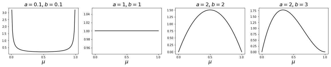
What sort of prior should we place on $\mu$? Let’s make two modeling assumptions. First, let’s assume that most coins are fair. This means that $\mu = 0.5$ should be the mode of the distribution. And let’s assume that biased coins do not favor heads over tails or vice versa. This means we want a symmetric distribution. One distribution that may have these properties is the beta distribution, given by

$\text{Beta}(\mu \mid a, b) = \frac{\Gamma(a + b)}{\Gamma(a) \Gamma(b)} \mu^{a-1} (1-\mu)^{b-1} \tag{2}$

where $\Gamma(x)$ is the gamma function

$\Gamma(x) = \int_{0}^{\infty} \mu^{x-1} e^{-\mu} \text{d} \mu$

and $\frac{\Gamma(a + b)}{\Gamma(a) \Gamma(b)}$ normalizes the distribution. The beta distribution is normalized so that

$\int_{0}^{1} \text{Beta}(\mu \mid a, b) \text{d} \mu = 1$

and has a mean and variance given by

$\begin{aligned} \mathbb{E}[\mu] &= \frac{a}{a+b} \\ \text{Var}(\mu) &= \frac{ab}{(a+b)^2 (a+b+1)} \end{aligned}$

The hyperparameters $a$ and $b$ (so-named because they are not learned like the parameter $\mu$) control the shape of the distribution (Figure $1$). Given our modeling assumptions, hyperparameters $a = b = 2$ seem reasonable.

Figure 1: The beta distribution for a variety of hyperparameters $a$ and $b$.

But another useful fact of the beta distribution—and the reason we picked it over the more obvious Gaussian distribution as our prior—is that it is conjugate to our likelihood function. Let’s see this. Let $l = n - m$ be the number of failures. If we multiply our likelihood (Equation $1$) by our prior (Equation $2$), we get a posterior that has the same functional form as the prior:

$\begin{aligned} p(\mu \mid m, l, a, b) &= \frac{\Gamma(a+b)}{\Gamma(a) \Gamma(b)} \mu^{a-1} (1-\mu)^{b-1} \prod_{i=1}^{n} \mu^{x_i} (1 - \mu)^{1 - x_i} \\ &\propto \mu^{m+a-1} (1-\mu)^{l+b-1} \end{aligned}$

Note that we only care about proportionality because $\Gamma(a+b)\,/\,\Gamma(a) \Gamma(b)$ is a constant that is independent of the parameter we want to learn and our data. We can see that our posterior is another beta distribution, and we can easily normalize it:

$p(\mu \mid m, l, a, b) = \frac{\Gamma(m+a+l+b)}{\Gamma(m+a)\Gamma(l+b)} \mu^{m+a-1} (1-\mu)^{l+b-1} \tag{3}$

Finally, we now want to maximize Equation $3$ rather than Equation $1$. Recall that this is maximum a posteriori (MAP) estimation because, unlike maximum likelihood estimation, we account for a prior. Because this new posterior is in a tractable form, it is straightforward to compute $\mu_{\text{MAP}}$. Let’s first compute the derivative of our new log likelihood with respect to $\mu$:

$\begin{aligned} \log p(\mu \mid m, l, a, b) &= \log(C) + (m + a - 1) \log(\mu) + (l + b - 1) \log(0 - \mu) \\ \frac{\partial}{\partial \mu} \log p(\mu \mid m, l, a, b) &= \frac{m + a - 1}{\mu} - \frac{l + b - 1}{1 - \mu} \end{aligned}$

where $C$ is the normalizing constant as in the previous section. Setting this equal to $0$ and doing some algebra, we get

$\mu_{\text{MAP}} = \frac{m + a - 1}{n + a + b - 2} \tag{4}$

Note that if $n = m = 0$, then $\mu_{\text{MAP}} = \frac{1}{2}$. In words, if we can’t flip a coin to estimate its bias, then the best we can do is assume the bias is the mode of our prior. And recall our small pathological example from before, the scenario when both $n = 3$ and $m = 3$. With our prior with hyperparameters $a = b = 2$, we have

$\mu_{\text{MAP}} = \frac{3 + 2 - 1}{3 + 2 + 2 - 2} = \frac{4}{5}.$

This demonstrates why the prior is especially important for parameter estimation with small data and how it helps prevent overfitting.

Benefits of conjugacy

I want to discuss two main benefits of conjugacy. The first is analytic tractability. Computing $\mu_{\text{MAP}}$ was easy because of conjugacy. Imagine if our prior on $\mu$ was the normal distribution. We would have had to optimize

$p(\mu \mid m, l, \sigma^2, \nu) = \frac{1}{\sqrt{2 \pi \sigma^2}} \text{exp} \Big(\frac{-(\mu - \nu)^2}{2 \sigma^2}\Big) \prod_{i=1}^{n} \mu^{x_i} (1 - \mu)^{1 - x_i}$

where $\sigma^2$ and $\nu$ are hyperparameters for the normal distribution. In the absence of techniques such as variational inference, conjugacy makes our lives easier.

The second benefit of conjugacy is that it lends itself nicely to sequential learning. In other words, as the model sees more data, the posterior at step $t$ can become the prior at step $t+1$. We simply need to update our prior and re-normalize. For example, imagine we process individual coin flips one at a time. Every time we see a heads ($x_i = 1$), we increment $n$ and $m$. Otherwise, we increment $n$ and $l$. Alternatively, we could fix $n = m = l = 0$ and just increment $a$ and $b$ respectively (Equation $4$).

Using this technique, we can visualize the posterior over sequential observations (Figure $2$).

Figure 2: Visualizing the posterior distribution (Equation $3$) for $n$ samples in $\{0, 10, 20, 30\}$. As the model sees more data, the posterior places more density around the true bias from the generative process. And after each data point, the posterior becomes the new prior.

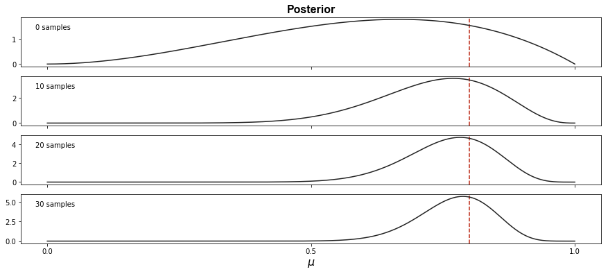
The upshot is that the posterior distribution becomes more and more peaked around the true bias as our model sees more data. Note that the $y$-axes are at different scales and therefore the last frame is even more peaked than the second-to-last frame. Also note that the posterior is slightly underestimating the true parameter $\mu = 0.8$, possibly because of the influence of the prior.

Conclusion

Conjugate priors are an important concept in Bayesian inference. Especially when one wants to perform exact Bayesian inference, conjugacy ensures that the posterior is tractable even after multiplying the likelihood times the prior. And they allow for efficient inference algorithms because the posterior and prior share the same functional form.

As a final comment, note that conjugacy is with respect to a particular parameter. For example, the conjugate prior of a Gaussian with respect to its mean parameter $\mu$ is another Gaussian, but the conjugate prior with respect to its variance $\sigma^2$ is the inverse gamma. The conjugate prior with respect to the multivariate Gaussian’s covariance matrix is the inverse-Wishart, while the Wishart is the conjugate prior for its precision matrix (Wikipedia, 2019). In other words, the conjugate prior depends on the parameter of interest and what form that parameter takes.

Acknowledgements

I borrowed some of this post’s outline and notation from Bishop’s excellent introduction to conjugacy (Bishop, 2006). See pages $68-74$ specifically.