An Intuitive Explanation of Black–Scholes

The Black–Scholes formula is the crown jewel of quantitative finance. The formula gives the fair price of a European-style option, and its success can ultimately be measured by its impact on option markets. Before the formula’s publication in 1973 (Black & Scholes, 1973; Merton, 1973), option markets were relatively small and illiquid, and options were not traded in standardized contracts. But after the formula’s publication, option markets grew rapidly. The first exchange to list standardized stock options, the Chicago Board Options Exchange, was founded the same year that Black–Scholes was published. And today, options are a highly liquid, mature, and global asset class, with many different tenors, exercise rights, and underlying assets.

The financial and mathematical theory underpinning Black–Scholes is rich, and one could easily spend months learning the foundational ideas: continuous-time martingales, Brownian motion, stochastic integration, valuation through replication, and risk-neutrality to name just a few key concepts. But properly contextualized, the formula can be surprisingly inevitable. It can almost feel like a law of nature rather than a financial model. My goal here is to justify this claim.

To begin, let’s setup the problem and then state the formula. Recall that a call option ($C$) is a contract that gives the holder the right but not obligation to buy the underlying asset ($S$) at an agreed-upon strike price ($K$). A put option ($P$) is the right but not obligation to sell the underlying short, but since calls and puts are fungible through put–call parity, we will only concern ourselves with call options in this post. If we can price one, we can price the other. We say the holder exercises the option if they choose to buy or sell the underlying. A European-style option can only be exercised at a fixed time in the future, called expiry ($T$).

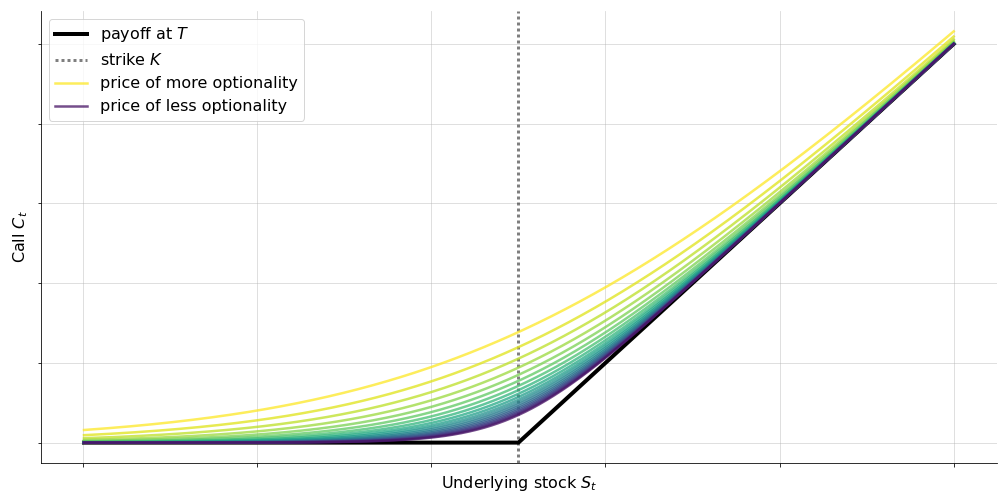
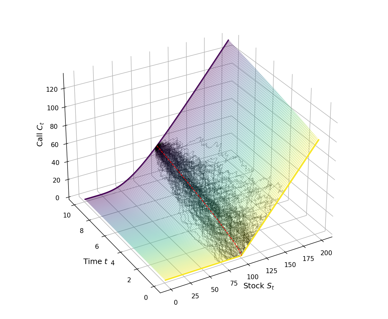
Clearly, the payoff at expiry of a European-style option is just a piecewise linear ramp function,

$\text{payoff of $C_T$} = \max\left[0, S_T - K\right], \tag{1}$

where $S_T$ denotes the value of the stock at expiry (black line, Figure $1$). The single most important characteristic of an option is this asymmetric payoff. For a call option, our downside is limited, but our upside is unlimited. In finance, this kind of asymmetric behavior is called “convexity”.

Given this, we might guess that the price of the call before expiry, so $C_t$ where $t \lt T$, should look like a smooth approximation of the ramp function (colored lines, Figure $1$), at least to a first approximation. Why? Imagine we hold a call before expiry, but the underlying $S_t$ is currently less than the strike $K$. Our position is not worthless precisely because it’s still possible that the stock price will rise before expiry. So we should still be able to sell the contract for more than zero. The closer the stock $S_t$ is to the strike $K$, the more we should be able to re-sell our option for. Put differently, and this is the key point here, the price of the option will change nonlinearly with the price of the stock, and as time passes, the smooth approximation should look more and more like the payoff function, because the option is losing its optionality.

Figure 1. The price of optionality (colored lines) should be always above the payoff of an option (black line) because the option could be worth something if the underlying price changes. More optionality (higher underlying volatility, more time to expiry) should be priced higher than less optionality. As time passes, an option loses its optionality and converges towards the payoff at expiry.

This tension between time decay and convexity is the central dynamic of an option, and the Black–Scholes formula encapsulates this tension beautifully. According to the Black–Scholes model, the fair price of a European-style call option is the following:

$\begin{aligned} C_t &= S_t \Phi(d_1) - K e^{-r(T-t)} \Phi(d_2), \\ d_1 &:= \frac{1}{\sigma \sqrt{T-t}} \left[ \log(S_t/K) + \left(r + (1/2) \sigma^2 \right) (T-t) \right], \\ d_2 &:= d_1 - \sigma \sqrt{T-t}. \end{aligned} \tag{2}$

Here, $\Phi(x)$ is the cumulative distribution function (CDF) of the standard normal distribution, $\sigma$ is the standard deviation or volatility of the underlying asset, and $r$ is the risk-free interest rate. Black–Scholes assumes that the volatility $\sigma$ and risk-free rate $r$ are both constant.

At a high level, this formula is just the weighted difference between the stock and strike prices. But the terms $\Phi(d_1)$ and $\Phi(d_2)$ are not obviously interpretable. So can we make headway here? Can we say something more precise without quickly getting bogged down in mathematical details? Let’s try.

Technical difficulties

Understanding how to derive Equation $2$ from first principles requires a complex set of mathematical and financial ideas. Perhaps the trickiest part for most people is the use of stochastic calculus (Itô, 1944; Itô, 1951; Bru & Yor, 2002). Stochastic calculus is required because we assume the underlying stock price follows this stochastic differential equation (SDE), which is a geometric Brownian motion:

$\frac{\text{d} S_t}{S_t} = \mu \text{d}t + \sigma^2 \text{d} Z_t. \tag{3}$

Here, $\mu$ is the drift of the stock, and $\sigma$ is the volatility of the stock. This is the same variable in as Equation $2$. Finally, $\text{d}Z_t$ is an infinitesimal change in a Brownian motion.

The important but subtle point here is that Equation $3$ is mathematically imprecise to most people, even those with strong technical backgrounds. In standard calculus, we cannot take the derivative of a random function. Informally, it breaks the required assumption that the function is smooth enough and can therefore be locally approximated by a tangent line. Thus, the notation $\text{d} Z_t$ has no meaning in standard calculus. So it appears that to even understand the generative model above, one must understand stochastic calculus.

As an aside, it’s worth mentioning that this technical difficulty is made even more subtle in the original paper (Black & Scholes, 1973) because it’s only a technical detail. The main content of the paper is the derivation of the famous Black–Scholes partial differential equation (PDE), and this is done by reasoning about the dynamics of an option. But since an option’s price is a function of its underlying stock’s price, describing its dynamics via a PDE requires partial derivative such as

$\frac{\partial C_t}{\partial S_t}. \tag{4}$

And of course, computing this term requires stochastic calculus since $S_t$ is a random function. So without stochastic calculus, any derivation of the Black–Scholes PDE is high-level at best. My approach in this post is to circumvent the PDE entirely and to just make sense of Equation $2$ directly. The PDE is beautiful—and perhaps I’ll write a separate post about it in the future—but we can still make progress by just thinking about the generative model of the stock price in simple, probabilistic terms.

Lognormally distributed prices

So let’s side-step the challenge of stochastic calculus implicit in Equation $3$. The key point is this: a differential equation is an equation that expresses the relationship between a function and its derivatives. And a solution here is the closed-form expression of $S_t$ such that we could plug $S_t$ and its derivative(s) into Equation $3$ and it would hold. A standard result is that the solution to the SDE in Equation $3$ is the following definition of $S_t$:

$S_t = S_0 \exp\left\{ \left( \mu - \frac{1}{2} \sigma^2 \right) t + \sigma Z_t \right\}, \quad Z_t \sim \mathcal{N}(0, t). \tag{5}$

If you want more detail, read about solving the SDE of geometric Brownian motion. But the main idea for us is that the Black–Scholes modeling assumption can be expressed in a form that does not require stochastic calculus. Equation $3$ can be reframed as the assumption that stock prices are lognormally distributed or, put differently, that log returns are normally distributed:

$\log S_t - \log S_0 \sim \mathcal{N}\left(\mu t - \frac{1}{2} \sigma^2 t, \sigma^2 t \right). \tag{6}$

So as a pedagogical trick, let’s just assume Equations $5$ and $6$ rather than Equation $3$. This is our new starting point.

For some intuition for the leap between the two, recall that the derivative of $\log x$ is $\frac{1}{x}\text{d}x$, and this looks a bit like the left-hand side of Equation $3$. So think of the left-hand side of Equation $3$ as a log return. And think of the right-hand side of Equation $3$ as a normally distributed random variable, since it is an incremental (additive) change in Brownian motion plus a constant drift. The extra term, $-(1/2) \sigma^2 t$, can only be properly understood with stochastic calculus—it’s from the quadratic variation of Brownian motion—, but it provides no real intuition for us here, and we will take it as a given.

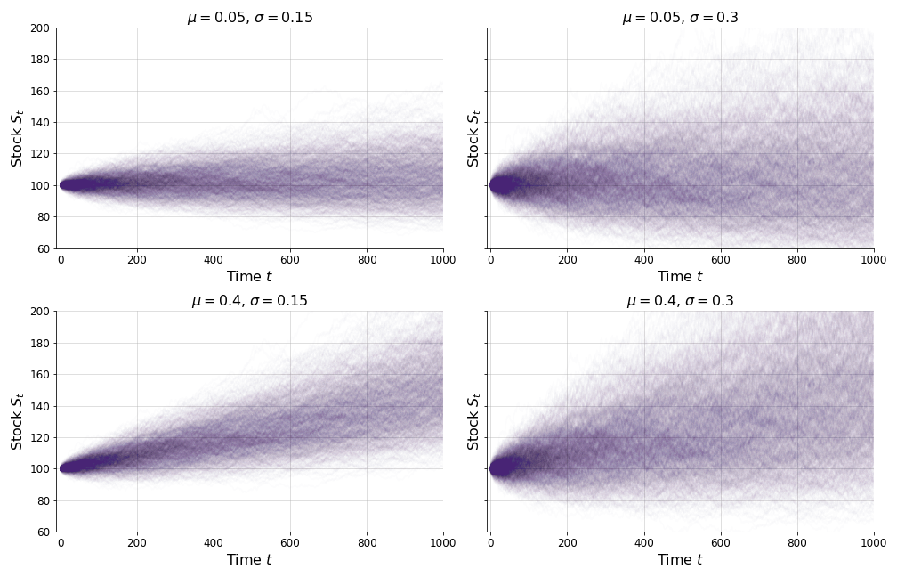
Let’s look at some examples. In Figure $2$, I have plotted the stock price over varying drifts $\mu$ and volatilities $\sigma$. This looks like random noise with drift because that’s precisely what it is. The normal distribution is as random as it gets, in the sense that the Central Limit Theorem states that the appropriately scaled sum of independent random variables converges to the normal distribution. Things that aren’t initially normal can still become normal over time.

Figure 2. Thousands of random samples from geometric Brownian motion with an initial stock price $S_0 = 100$ and varying drifts and volatilities.

Now if $\log S_t$ is normally distributed, then $S_t$ is lognormally distributed. So as time $t$ passes, the stock price $S_t$ is always lognormally distributed with a variance that increases linearly with time and thus a volatility that increases with the square root of time. To visualize this assumption, I’ve plotted the appropriate lognormal distribution at various time slices along with a many empirical samples (Figure $3$). In my mind, this figure captures the geometric essence of Equations $3$ and $5$. Black–Scholes assumes that the stock price is unpredictable modulo the drift, and that “infinitesimal change in Brownian motion”, mathematically vague for the uninitiated, amounts to an uncertainty about the stock price that grows with the square root of time.

Figure 3. Thousands of random samples from geometric Brownian motion with an initial stock price $S_0 = 100$, drift $\mu = 0.2$, and volatility $\sigma = 0.15$. The lognormal distribution at various time points (Equation $6$) is plotted in dashed black lines.

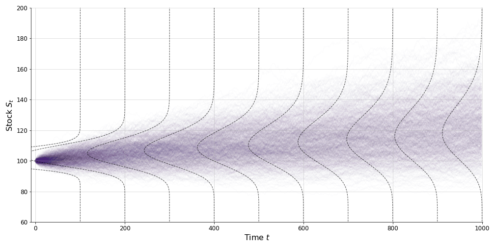
Of course, we could make the same figure but using log returns. In that case, the lines indicating the lognormal distributions in Figure $3$ would change to indicate normal distributions. In either case, the generative model of Black–Scholes is that prices and therefore returns are unpredictable.

Now pause. We’re going to make a subtle but critical tweak to our assumptions so far. We’re going to replace the stock-specific drift $\mu$ with the risk-free interest rate $r$. Concretely, rather than assuming Equation $6$, we’re going to assume a stock’s log returns follow this normal distribution:

$\log S_t - \log S_0 \sim \mathcal{N}\left(r t - \frac{1}{2} \sigma^2 t, \sigma^2 t \right). \tag{7}$

We haven’t discussed $r$ in detail yet, but this is just the an idealized number representing the time-value of money. To a first order, think of $r$ as the interest rate from a very secure or reliable asset, such as a short-term US government bond. It is the risk-free rate and thus the lower-bound on what you can earn without risk.

Of course, different stocks might be modeled with different drifts. The drift of a blue-chip company might not be the same as the drift of a penny stock. So in essence, this assumption is a claim that Black–Scholes is making: the drift of the stock doesn’t matter when pricing an option! This is a surprising and deep claim. Let’s understand it.

Risk neutral world

In the original paper, Black and Scholes assume that the market has no arbitrage. Here, an “arbitrage” is an opportunity to make a risk-free profit starting at zero wealth. In other words, Black–Scholes assumes the market is perfectly efficient, and the formula (Equation $2$) represents the fair price of the option in this idealized world.

Now when I first learned this stuff, I found this assumption confusing, because I thought it was analogous to assuming “no friction” in a high-school physics problem. In physics, we might simplify the world by assuming that a box slides on plane without friction. This makes calculations easier for students, but the consequence is that predictions are systematically wrong. At some point, we have to add friction back into our model to make it realistic.

But friction is a poor analogy here, and I propose a different one: assuming no arbitrage is analogous to assuming no wind or air resistence when modeling projectile motion. This assumption also simplifies calculations, but really it helps us understand the essence of the phenomenon: the parabolic arc of projectile motion. Later, we can add air resistance or wind depending on our particular circumstances, but the underlying parabolic arc is a kind of platonic ideal. It is the signal without the noise.

This is the sense in which Black–Scholes assumes no arbitrage. The assumption is not an implausible claim that real financial markets are perfectly efficient. Rather, assuming no arbitrage is assuming a perfectly coherent, noise-free system where prices are consistent and make sense relative to each other. So this isn’t about simplifying calculations. It’s about finding the platonic price. And thus it’s not an assumption that we remove in the future to get a more realistic price. Quite the opposite! Adding arbitrage would make the problem impossible to solve because prices would then be inconsistent. There would be no universally agreed-upon market price.

Now that we understand this, let’s retrace the main line of argument of the original paper (Black & Scholes, 1973), but let’s do so in a simpler context. Imagine we sold a hypothetical derivative contract: a redeemable certificate on a stock, which can be exercised only at time $T$. An investor pays us $R_0$, the fair price of the redeemable at inception, and in return we give them a certificate that is redeemable for the value of the stock at time $T$. Our goal is to solve for $R_t$, the fair price of the redeemable at any given moment in time.

As dealers, the risk to us is that the price of the stock goes up. So what could we do? Well, the moment we sell a redeemable, we could buy the underlying stock. Now we are perfectly hedged. We don’t care if the stock goes up or down in value, because we own the stock. Whenever a customer comes to redeem the value of the stock, we simply sell the appropriate share, and we’re done. We neither make nor lose money on average, and thus the price is fair.

The key insight of Black–Scholes is to realize that our perfectly hedged portfolio, short a redeemable and long a stock, is risk-less. And thus, it must grow or drift at the risk-free rate! Formally, we can say that the value of our portfolio at expiry $T$ is

$S_T - R_T = e^{rT} (S_0 - R_0). \tag{8}$

This is remarkable because $S_T$ is random! But the left-hand side is not an expectation, because we are always hedged! Do you see the trick? This is the big idea of the original paper. We’ve neutralized the randomness in $S_t$ by assuming we can perfectly hedge it out!

Now a terminal condition is that our redeemable is worth the value of the stock at expiry, so $S_T = R_T$. This is fair in the sense that neither we nor the investor makes more money than the other. Under this condition, we can write Equation $8$ as

$e^{rT} R_0 = e^{rT} S_0. \tag{9}$

But if our portfolio is perfectly hedged and riskless, then clearly $R_0$ must be a riskless derivative. And so it must drift at the risk-free rate, giving us

$R_T = e^{rT} S_0. \tag{10}$

And of course, we can replace big $T$ with little $t$, in general. Doesn’t this make sense? The fair price of the redeemable is simply the price of the stock at contract inception, adjusted for the time-value of money! Again, despite $S_t$ being a random process, we have no expectations. We have neutralized randomness through perfect hedging in a world without arbitrage.

Now let’s extend this line of reasoning to options. The challenge here is that an option has convexity. Its price changes nonlinearly with changes in the underlying. So unlike with the redeemable, we would not want to buy exactly one share of stock for one option contract. Instead, at each moment, we want precisely the amount of stock such that, if the stock price moved an infinitesimally small amount, our hedge would move an infinitesimally small amount that perfectly matched the price of the option. This sounds like a derivative from calculus because it is! The amount we want to hedge at an instant in time is simply the derivative of the call price with respect to the stock price, called the delta:

$\text{delta} := \Delta_t = \frac{\partial C_t}{\partial S_t}. \tag{11}$

So if the stock changes by one dollar, our option price changes by approximately $\Delta_t$ dollars.

Now imagine a world without arbitrage or transaction fees and with continous trading. In this world, we (an options dealer) can always be perfectly delta hedged. Our portfolio is always just

$\Delta_t S_t - C_t. \tag{12}$

In the original paper, the authors repeat the argument made above for redeemables but in the context of options. The calculations become more complicated because working with $\Delta_t$ requires stochastic calculus, since $S_t$ is a random variable. But the argument is essentially the same. We assume a world without arbitrage and then just model the dynamics of a perfectly hedged and thus risk-less portfolio. We use these dynamics (Black–Scholes PDE) and a terminal condition to solve for the fair price $C_t$.

That’s the original argument. It’s an argument about no arbitrage and perfect hedging. But Black–Scholes feels like a law of nature because it’s the solution to a noise-free system and because it can be derived in many ways. Another way to derive Black–Scholes is by modeling a portfolio which perfectly replicates the price of a call at each moment. This idea of valuation through replication is far-reaching in finance. To quote Emanuel Derman (Derman, 2002):

If you want to know the value of a security, use the price of another security that’s as similar to it as possible. All the rest is modeling.

The discrete-time version of this argument is the binomial options-pricing model. Yet another way is to connect the idea of no arbitrage to the idea of risk-neutrality. This relationship is called the fundamental theorem of asset pricing, and it’s the relationship we want to explore here.

(As an aside, in my mind, one of the confusing things about many presentations of Black–Scholes is that presenters will seemlessly switch between these different arguments, without acknowledging that it is non-obvious that they are equivalent and without acknowledging which line of argument Black, Scholes, and Merton used.)

Let’s understand this connection between the original argument of no arbitrage and the modern argument of risk-neutral pricing. Consider this: in a Black–Scholes world, do we care about the drift of the underlying stock? As with a redeemable, we are always perfectly and continuously delta hedged. We have no price exposure. In this world, all options dealers would perfectly hedge. And all options investors would become risk-neutral, because it would not pay to take risk. So one trick that makes our logic and calculations easier is to just assume the drift of the stock is $r$! This is equivalent to assuming the world has no arbitrage. And what’s the fair price of an option in this world? It’s a time-discounted expected value:

$C_t = e^{-r(T-t)} \mathbb{E}_{\mathbb{Q}} \left[\max[0, S_t - K]\right]. \tag{13}$

Here, the subscript $\mathbb{Q}$ is called the risk-neutral measure, and this notation is used to make it explicit that the expectation is computed in this imaginary world, not in the real risky world. In this imaginary world, $S_t$ is a martingale, which is a stochastic process with an expected value that is always equal to the current value. Intuitively and importantly, martingales have no drift. So in Equation $13$, the only drift is from the discount factor $e^{-r(T-t)}$. The stock itself is a drift-less martingale.

So in one telling, we assume the world has no risk, and thus we can work without expectations. Random processes can be forced to become non-random. In another telling, we assume the world is risk-neutral, and random processes become martingales. In both tellings, the only meaningful drift is the risk-free rate.

There is a lot of theory one could get into here. For example, the Girsanov theorem is a result from probability theory on how a stochastic process changes under a change in measure (here, from the true “physical” measure to the risk-neutral measure). And you might read things like, “Under the risk-neutral measure, the stock price after discounting by the risk-free rate follows a martingale”. You can easily get lost in the technical details. But in my mind, at a high-level, the concept is fairly simple, if a bit non-obvious. In a world in which all investors and traders can perfectly hedge their risk, there is no risk premia; everyone is forced to become risk neutral. And thus, the price of everything is its risk-neutral expected value, or its value if there was no premia to risk.

And again, this simplifying assumption is not like assuming “no friction”. We do not need to re-add arbitrage or drift in order to compute a more realistic option price later. Instead, this assumption strips out all the noise, and $C_t$ represents a platonic price in a coherent and consistent market.

Armed with this understanding, let’s revisit the generative model for a stock. In a risk-neutral world, the drift of every stock is the same: it’s just the risk-free rate $r$. This is the line of reasoning which converts Equation $6$ to Equation $7$.

Contingent values

We’re now ready to try to directly make sense of Equation $2$. At this point, we’ll need to a bit of tedious algebra, but nothing in this section requires more than basic probability. And the conceptual work is mostly done. As promised, I’ve tried to side-step as much stochastic calculus as possible in order to get to this point.

For easy access, let’s repeat the main formula:

$\begin{aligned} C_t &= S_t \Phi(d_1) - K e^{-r(T-t)} \Phi(d_2), \\ d_1 &:= \frac{1}{\sigma \sqrt{T-t}} \left[ \log(S_t/K) + \left(r + (1/2) \sigma^2 \right) (T-t) \right], \\ d_2 &:= d_1 - \sigma \sqrt{T-t}. \end{aligned} \tag{14}$

Let’s also repeat our modeling assumption (Equation $7$) but in terms of $T$ and $t$:

$\begin{aligned} \log S_T - \log S_t &\sim \mathcal{N} \left(m, s^2\right), \\ m &:= \left( r - \frac{1}{2} \sigma^2 \right) \tau, \\ s &:= \sigma \sqrt{\tau}, \\ \tau &:= T - t. \end{aligned} \tag{15}$

As a final preliminary, two observations for notational clarity. First, note that at time $t$, the price $S_t$ is non-random. So we can push that into the mean if we would like, giving us:

$\log S_T \sim \mathcal{N}\left(\log S_t + m, s^2 \right). \tag{16}$

Second, here I’ve used notation $d_1$ and $d_2$ to match what I have commonly seen in the literature. But I think it’s extremely useful to rewrite $d_2$ as

$\begin{aligned} d_2 &= d_1 - \sigma \sqrt{\tau} \\ &= \frac{\log(S_t/K) + \left(r + (1/2) \sigma^2 \right) \tau - \sigma^2 \tau}{\sigma \sqrt{\tau}} \\ &= -\frac{\log(K/S_t) - \left(r - (1/2) \sigma^2 \right) \tau}{\sigma \sqrt{\tau}} \\ &= -\frac{\log(K/S_t) - m}{s}. \end{aligned} \tag{17}$

We’ll use this momentarily.

Now at a high-level, my claim is that we can think of $C_t$ as decomposable into two terms, one representing what we make (stock price) and one representing what we pay (strike price), both contingent on the call ending in-the-money ($S_T \gt K$). This idea is not original to me; it is from (Nielsen, 1992). We have:

$\begin{aligned} C_1 &= \text{contigent value of stock} &&= \begin{cases} S_T & \text{if $S_T \gt K$,} \\ 0 & \text{else,} \end{cases} \\ \\ C_2 &= \text{contigent value of strike} &&= \begin{cases} -K & \text{if $S_T \gt K$,} \\ 0 & \text{else.} \end{cases} \end{aligned} \tag{18}$

Furthermore, both of these terms will have a clear, simple, probabilistic interpretation that will directly map onto Equation $14$. Let’s see this.

First, what is $\mathbb{E}[C_2]$? This is an expectation, and the value of the claim is zero when the call is out-of-the-money (when $S_T \lt K$). By definition:

$\begin{aligned} \mathbb{E}[C_2] &= 0 \times \mathbb{P}(S_T \lt K) + (-K) \times \mathbb{P}(S_T \gt K) \\ &= -K \times \mathbb{P}(S_T \gt K). \end{aligned} \tag{19}$

And it is easy to see that $\mathbb{P}(S_T \gt K)$ is equal to $\Phi(d_2)$!

$\begin{aligned} \mathbb{P}(S_T \gt K) &= \mathbb{P}(\log(S_T / S_t) \gt \log(K / S_t)) \\ &= \mathbb{P} \left( \frac{\log(S_T/S_t) - m}{s} \gt \frac{\log(K/S_t) - m}{s} \right) \\ &= \mathbb{P} \left( Z_T \gt -d_2 \right) \\ &= 1 - \mathbb{P}(Z_T \lt -d_2) \\ &= \mathbb{P}(Z_T \lt d_2) \\ &= \Phi(d_2). \end{aligned} \tag{20}$

Here, $Z_T$ denotes the $z$-score of the log move from $S_t$ to $S_T$, i.e.

$Z_T := \frac{\log(S_T/S_t) - m}{s} \sim \mathcal{N}(0, 1). \tag{21}$

So in words, we can see that $\Phi(d_2)$ is just the probability that the call ends up in-the-money, or the probability that $S_T \gt K$. All those extra variables embedded in $d_2$ just represent normalizing the log move from $S_t$ to $S_T$, such that we can represent the equation using the CDF of the standard normal rather than the CDF of $S_T$. We could, if we wanted to, represent all of this using the CDF of the un-standardized lognormal distribution. But it’s cleaner and conventional to work in a standardized space.

To summarize, we have shown:

$\text{expected contingent value of strike} = \mathbb{E}[C_2] = -K \Phi(d_2). \tag{22}$

This represents the expected value we must pay to exercise a call option, contingent on the option being exercised. Of course, this is an expected value, but the Black–Scholes price is the price in today’s terms. So we need a discount factor, giving us:

$\text{$\mathbb{E}[C_2]$ at time $t$} = -e^{-r(T-t)} K \Phi(d_2). \tag{23}$

Now for $C_1$, we again have an expectation where the contingent value is zero when the option ends out-of-the-money. This is a bit more complicated than the derivation for $C_2$, since $S_T$ is random while $K$ is fixed. By the law of total expectation, we have:

$\begin{aligned} \mathbb{E}[C_1] &= 0 \times \mathbb{P}(S_T \lt K) + \mathbb{E}[S_T \mid S_T \gt K] \times \mathbb{P}(S_T \gt K), \\ &= \mathbb{E}[S_T \mid S_T \gt K] \mathbb{P}(S_T \gt K). \end{aligned} \tag{24}$

While this is a bit trickier, it’s still relatively straightforward to put into words. It is the weighted average contribution of the expected stock price, conditional on the fact that we exercise the call. Since $S_T$ is lognormally distributed (Equation $16$), we can write this expectation in terms of a truncated lognormally distributed random variable $\hat{S}_T$:

$\hat{S}_T = \begin{cases} S_T & \text{if $S_T \gt K$}, \\ 0 & \text{else}. \end{cases} \tag{25}$

And coincidentally, I recently wrote a blog post on the expected value of the truncated lognormal distribution! Using the parameters $m$ and $s$ from Equation $15$ here and plugging them into Equation $15$ in that blog post, we can easily compute the expectation:

$\begin{aligned} \mathbb{E}[\hat{S}_T] &= \mathbb{E}[S_T \mid S_T \gt K] \\ &= \frac{\mathbb{E}[S_T] \Phi\left( s - \frac{\log K - (\log S_t + m)}{s} \right)}{1 - \Phi\left(\frac{\log K - (\log S_t + m))}{s}\right)}. \end{aligned} \tag{26}$

And denominator is the probability that we exercise the call!

$1 - \Phi\left(\frac{\log K - (\log S_t + m))}{s}\right) = 1 - \Phi(-d_2) = \Phi(d_2) = \mathbb{P}(S_T \gt K). \tag{27}$

Putting this together, we can see that we can rewrite Equation $24$ as:

$\begin{aligned} \mathbb{E}[C_1] &= \mathbb{E}[S_T \mid S_T \gt K] \mathbb{P}(S_T \gt K) \\ &= \mathbb{E}[S_T] \Phi\left( s - \frac{\log(K/S_t) - m)}{s} \right) \\ &= \mathbb{E}[S_T] \Phi\left( s + d_2 \right) \\ &= \mathbb{E}[S_T] \Phi\left( d_1 \right). \end{aligned} \tag{28}$

This looks very promising, and we can solve this because we also know the expected value of a lognormally distributed random variable. It’s

$\begin{aligned} \mathbb{E}[S_T] &= \exp\left\{ \log S_t + m + \frac{1}{2} s^2 \right\} \\ &= S_t \exp\left\{ \left(r - \frac{1}{2} \sigma^2\right) \tau + \frac{1}{2} \sigma^2 \tau \right\} \\ &= S_t e^{r (T-t)}. \end{aligned} \tag{29}$

Now that both makes sense in a risk-neutral world, and it looks quite promising. This means we have shown

$\mathbb{E}[C_1] = e^{r (T-t)} S_t \Phi(d_1). \tag{30}$

And once again, we need to discount this for the current time, giving us:

$\text{$\mathbb{E}[C_1]$ at time $t$} = S_t \Phi(d_1). \tag{31}$

That’s it. We’re done. This is a simple, probabilistic interpretation of the Black–Scholes formula. To summarize, it is the difference between two contingent values:

$\begin{aligned} C_t &= e^{-r(T-t)} \left[ \mathbb{E}[C_1] + \mathbb{E}[C_2] \right] \\ &= S_t \Phi(d_1) -e^{-r(T-t)} K \Phi(d_2). \end{aligned} \tag{32}$

In more words, the left term is the time-discounted and weighted-average expected value of the stock, contingent on exercising. And the right term is the time-discounted expected value of the strike, again contingent on exercising. The main conceptual hurdle was realizing why we needed to replace the stock-specific drift $\mu$ with the risk-free rate $r$. But once we understood that, we could assume that the underlying stock’s log returns were normally distributed as in Equation $15$. Everything else was just computation.

Figure 4. Thousands of random samples from geometric Brownian motion as in Figure $3$ but truncated at strike $K=95$. The truncated lognormal distribution at various time points is plotted in dashed black lines. The mean of these distributions (dashed purple line) is the mean of the truncated lognormal. The term $S_t \Phi(d_1)$ is just this mean weighted by $\mathbb{P}(S_T \gt K)$.

In my mind, this view of Black–Scholes finally helped me understand $\Phi(d_1)$. While $\Phi(d_2)$ has a clean interpretation—it’s just the probability that the call is exercised (Equation $20$)—I initially found $\Phi(d_1)$ less clear. But perhaps my confusion was due to my attempt to understand the term in isolation. Really, I think it helps to think about $S_t \Phi(d_1)$ as a single unit. This represents the weighted-average present value of the stock, contingent on the option ending in the money (Equations $28$ and $29$).

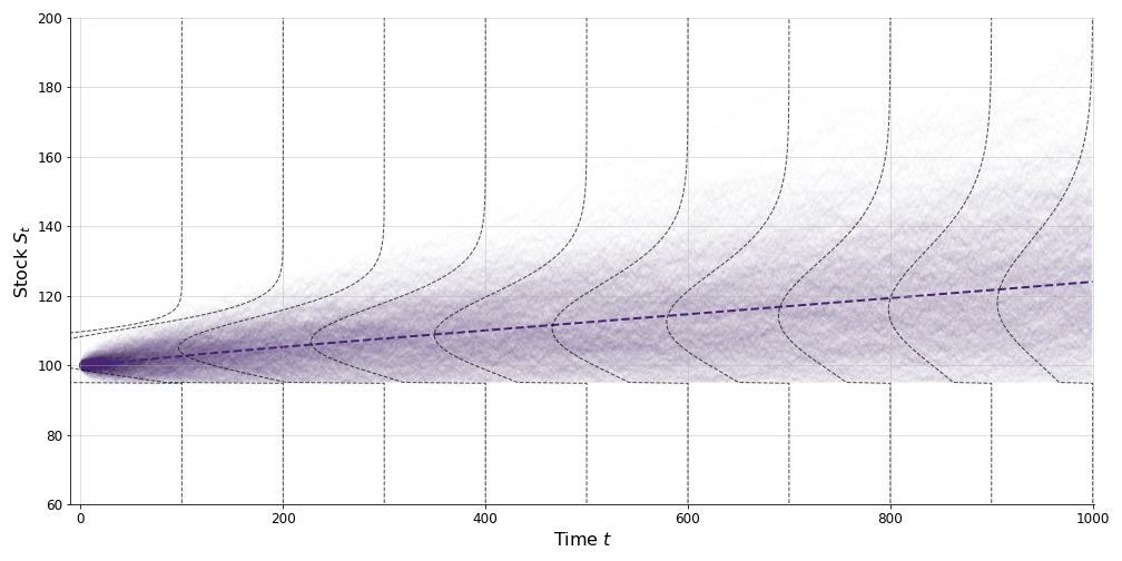
I think this has a nice geometric interpretation. We can think of the contingent value of our stock as following a truncated lognormal distribution (Figure $4$). Here, $S_t \Phi(d_1)$ is the expected value of this truncated lognormal random variable, weighted by the probability that the call is exercised.

Conclusion

As a final sanity check, I’ve visualized the Black–Scholes price for a call option across various times to expiry (Figure $5$). Again, we see the inherent tension between time-decay and convexity. As time passes, an option loses value as it loses optionality, but it gains value as it gains convexity. Ultimately, the Black–Scholes PDE models this tension directly.

In this post, however, we side-stepped the PDE entirely in favor of an intuitive understanding of risk-neutrality. In a world without arbitrage, everyone can perfectly hedge their option positions, and thus everyone is risk-neutral. In this world, all stock prices are converted into martingales, stochastic process without drift or memory. In this world, the fair price of an option is just its time-discounted, risk-neutral expected value. And this discounted expected value has a clean interpration: it is the difference between two contingent values, the contingent value of the stock and the contingent value of the strike.

Figure 5. Visualization of the Black–Scholes formula for an initial stock price $S_0 = 100$, drift $\mu = 0.04$, and volatility $\sigma = 0.15$ over hundreds of samples. At each moment, the call gains or loses value, contingent on the stock price $S_t$ and the time to expiry $T-t$.

Hopefully this post justifies my original claim: Black–Scholes feels inevitable, like a natural law. It makes some very simplifying assumptions, such as constant volatility, but the model works extremely well in practice. Many decades later, investors, traders, and other market participants still use Black–Scholes daily. Much like other simple models such as linear regression, Black–Scholes is wrong but useful, interpretable, and general due to its simplicity. And it is the foundation and reference point for more complex models.