Square Root of Time Rule

Big idea

In finance, the riskiness of an asset is often defined by its volatility, which is itself quantified as the standard deviation of the asset’s returns. However, the magnitude of volatility is a function of the frequency of the data. Lower-frequency data will have bigger returns, since the price has more time to move between samples. Therefore, the volatility of lower-frequency data will typically be higher than the volatility of higher-frequency data.

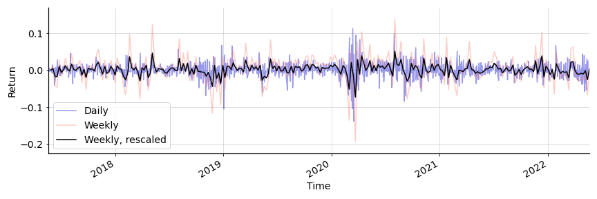
For example, consider Apple (AAPL) stock prices and returns, sampled daily and weekly (Figure $1$). Clearly, monthly prices will induce larger returns than daily prices. If we compute the standard deviation of the daily and weekly return series in Figure $1$, we get very different estimates of volatility: $0.0199$ and $0.0396$ respectively. Thus, we would like a way to time-aggregate volatility, so that we can compare and reason about the riskiness of assets at different frequencies.

Figure 1. (Top) Apple stock prices, reported at daily and weekly frequencies. (Bottom) Apple stock's log returns computed from their associated price series.

One way to handle this time aggregation is the square root of time rule, which is the heuristic that a higher-frequency volatility estimate can be scaled to a lower-frequency volatility estimate by multiplying by the square root of “time”. Here, “time” is the ratio between the number of high- to low-frequency samples.

For example, in Figure $1$, the ratio between the number of daily-to-weekly samples is $7$, since there are $7$ days in a week. Thus, to estimate weekly volatility from daily data, we would multiply the daily volatility by $\sqrt{7}$. To estimate daily volatility from weekly data, we would divide the weekly volatility by $\sqrt{7}$. Figure $2$ illustrates this computation by comparing daily returns to weekly returns that have been rescaled by $\sqrt{7}$. Now the rescaled weekly volatility is $0.0149$.

Figure 2. Daily and weekly log returns, along with weekly log returns rescaled by the square root of time. The rescaled weekly returns have movements that are roughly on the same scale as the daily returns.

As a second example, consider the Black–Scholes equation, which scales volatility by the square root of the time to maturity for an options contract.

Deriving the rule

So why does this calculation work? Any random variable that is the sum of independent and identically distributed random variables will have a variance that scales linearly with the number of random variables in the sum. This basic idea applies to many random processes that make independence assumptions.

For example, imagine a Gaussian random walk with $T$ steps, where each step $X_t$ is i.i.d. The total distance after $T$ steps is the random variable $Y_T$,

$Y_T = X_1 + X_2 + \dots + X_T, \qquad X_t \stackrel{\textsf{iid}}{\sim} \mathcal{N}(\mu, \sigma^2). \tag{1}$

Then the variance of $Y_T$ is

$\mathbb{V}[Y_T] = \sum_{t=1}^T \mathbb{V}[X_t] = T \mathbb{V}[X_1] = T \sigma^2,. \tag{2}$

and the volatility is

$\sqrt{T} \sigma. \tag{3}$

As a second example, in a Poisson process, the arrival time of the $T$-th element is the sum of $T$ exponentially distributed random variables,

$Y_T = X_1 + X_2 + \dots + X_T, \qquad X_t \stackrel{\textsf{iid}}{\sim} \text{exp}(\lambda). \tag{4}$

Here, each $X_t$ is the waiting time between any two arrivals from a Poisson distribution. The variance of $Y_T$ is

$\mathbb{V}[Y_T] = T \mathbb{V}[X_1] = \frac{T}{\lambda^2}. \tag{5}$

Again, this implies that the volatility of $Y_T$ scales with the square root of the number of random variables, $\sqrt{T}$.

At this point, you might be asking: how does any of this apply to the returns in Figures $1$ and $2$? If $X_t$ is a random variable representing the log return (not the raw return) of an asset, then the cumulative return $Y_T$ of buying an asset at time $t=1$ and holding it through time $T$ is simply the sum of these returns:

$Y_T = X_1 + X_2 + \dots + X_T. \tag{6}$

If you are unconvinced, see Equation $16$ in my previous post on log returns. Thus, when working with log returns, higher-frequency data can be time-aggregated into lower-frequency data by summing the log returns by into desired periods (e.g. weeks, months, years). In fact, this is precisely how I constructed Figures $1$ and $2$: I computed daily log returns from daily price data and then computed weekly log returns by summing data within each week. As we saw, these time-aggregated or cumulative returns have a higher volatility. If we’d like, we can normalize the volatility using the square root of time rule.

As a final note, some resources incorrectly claim that the data must be independent and normally distributed, but normality is not a required assumption, as can be seen above.

Conclusion

The square root of time rule is a heuristic for rescaling the volatility estimate of a particular time series to a new data frequency. The rule assumes that our data are the sum of i.i.d. random variables. This applies to many random processes used in finance. Even when these basic assumptions do not hold, scaling volatility by the square root of time can still be a useful heuristic for estimating volatility to a first approximation.