Returns and Log Returns

Prices and returns

Prices between assets may be difficult to compare. For example, a large company might have a higher stock price than a smaller competitor. However, the bigger company’s price could be relatively stable, while the competitor’s smaller price is rapidly increasing. Thus, it is natural to want to think of prices in relative terms. Let $p_t$ denote the price of an asset at time $t$. Then the return of an asset captures these relative movements and is defined as

$r_t = \frac{p_t - p_{t-1}}{p_{t-1}}. \tag{1}$

In words, a return is the change in price of an asset, relative to its previous value. Note that $p_t > 0$, and therefore $r_t > -1$. Equation $1$ can be rewritten as

$r_t = \frac{p_t}{p_{t-1}} - 1. \tag{2}$

For example, if $p_{t-1} = 100$ and $p_t = 110$, then the $r_t = 0.1$ or a return of $10\%$ in one time period.

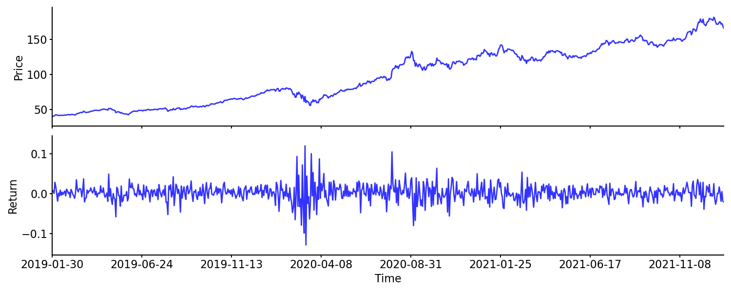
To highlight the difference between prices and returns, I have plotted the closing price and return of Apple Inc. (AAPL) for the past three years. Data is from Yahoo! Finance. We can see that AAPL returns were highest (and lowest) around March 2020, despite the closing price having a drawdown during that period.

Figure 1. AAPL closing prices (top) and returns (bottom) for the past three years.

Cumulative returns

Imagine we invest principal $p_0$ into an asset with return sequence $\{ r_1, r_2, \dots, r_T \}$. What is our cumulative return, assuming we buy at $t=0$ and sell after $t=T$, after realizing return $r_T$? For example, if we buy an asset for $$100$ and see a $10\%$, $5\%$, and then $-2\%$ return, our asset is worth

$100 (1.1) (1.05) (0.98) = 113.19 \tag{3}$

at time $T=3$. So $p_0 = 100$ and $p_T = 113.19$. So our total return is

$\frac{113.19}{100} - 1 \approx 0.13, \tag{4}$

or a $13\%$ return. Since we started with $p_0$ and since our return was $\prod_{t=1}^T (1 + r_t)$, our cumulative return was

$\frac{p_0 \prod_{t=1}^T (1 + r_t)}{p_0} - 1. \tag{5}$

This is just Equation $2$ over $T$ time periods:

$r_{0:T} = \frac{p_T}{p_0} - 1 = \prod_{t=1}^T (1 + r_t) - 1. \tag{6}$

Here, I use the notation $r_{i:j}$ with $i < j$ to refer to the cumulative return between periods $i$ and $j$.

Notice that we are letting our returns compound continuously, meaning we are reinvesting any gains between time periods. However, we may want to constantly rebalance our portfolio, so that we have a constant exposure $p_0$. What this means is that after each day (or time period), we either take a profit (if positive return) or buy more of the asset (if negative return) to ensure that we always have $p_0$ of the asset at the beginning of each period. In that case, after $T$ days, our profit (not return) is

$\omega_{1:T} = p_0 r_1 + p_0 r_2 + \dots + p_0 r_T = p_0 \left( \sum_{t=1}^T r_t \right). \tag{7}$

Here, I use $\omega$ rather than $p$ to disambiguate prices from profit. For example, if we invest $p_0 = 100$ into an asset, which then has returns $\{0.1, -0.05\}$, then our profit is

$100 (0.1) + 100 (-0.05) = 5. \tag{8}$

And our cumulative return with rebalancing is again similar to Equation $2$ for $T$ time periods:

$\begin{aligned} r_{0:T} &= \frac{p_0 + \omega_{1:T}}{p_0} - 1 \\ &= \frac{p_0 + p_0 \left(\sum_{t=1}^T r_t \right)}{p_0} - 1 \\ &= \sum_{t=1}^T r_t. \end{aligned}\tag{9}$

However, something subtle is happening here. Notice that our profit, $\omega_{1:T}$, can be negative, unlike prices. And while a single return $r_t$ is lower-bounded by $-1$, since prices are lower-bounded by zero, the return $r_{0:T}$ with rebalancing could be infinitely negative. This is because we could be reinvesting $p_0$ over an infinite series of negative returns.

To summarize, we have two kinds of cumulative returns:

$\begin{aligned} \text{cumulative return, compounding} &= \prod_{t=1}^T (1 + r_t) - 1, \\ \text{cumulative return, rebalancing} &= \sum_{t=1}^T r_t. \end{aligned} \tag{10}$

Which is being referred to often depends on context. However, for the remainder of this post, let’s focus on continuously compounded cumulative returns.

Log returns

In practice, “returns” often means “log returns”. Log returns are defined as

$z_t = \log(1 + r_t). \tag{11}$

This can be expressed in terms of $p_t$ and $p_{t-1}$ (as in Equation $2$) as

$z_t = \log\left( \frac{p_t}{p_{t-1}} \right). \tag{12}$

Let’s look at a few reasons why log returns are sometimes preferred over raw returns.

Infinite support

Returns are lower-bounded by $-1.0$. One cannot lose more than all of one’s money. However, log returns have an infinite support. And since the log function suppresses big positive values while emphasizing small negative values, log returns are more symmetric than returns. This is a natural consequence of logarithms (Figure $2$, left).

Figure 2. (Left) Graphs of $f(x) = x$ (red) and $f(x) = \log(1 + x)$ (blue). Note that the latter function is $\log(x)$ but shifted left by one such that it goes through the origin. (Right) Probability plot of returns and log returns from SNAP.

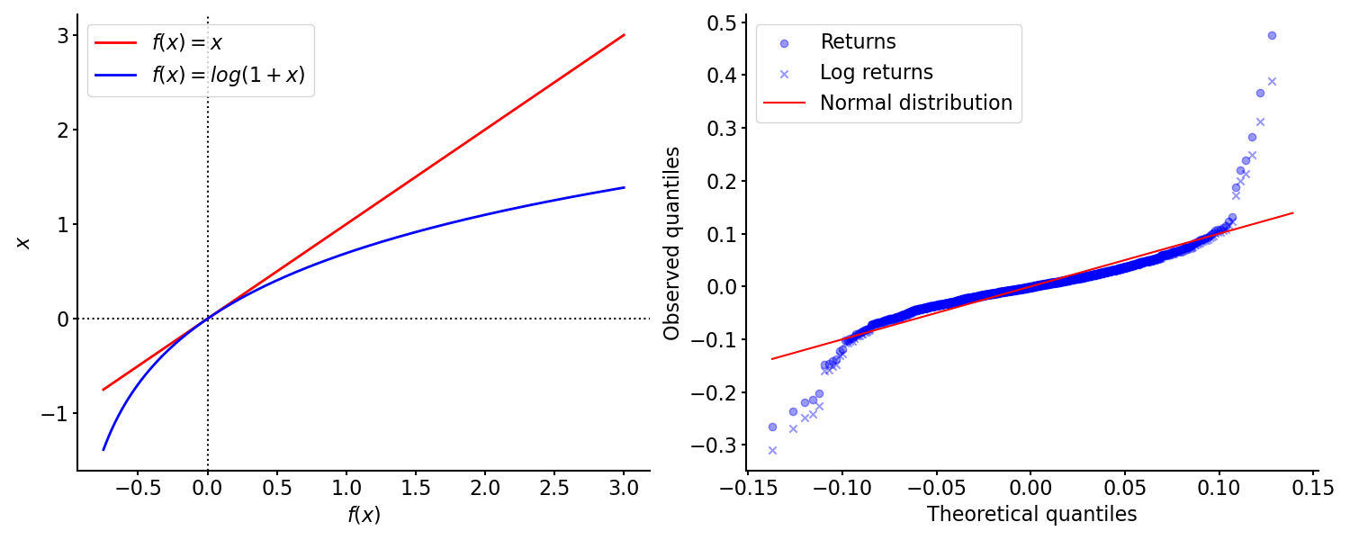
Another way to see this is to plot the theoretical quantiles of a symmetric distribution against the observed quantiles of our data. This is sometimes called a probability plot. In Figure $2$ (right), I’ve created a probability plot for Snap Inc. (SNAP) returns using the normal distribution as the theoretical distribution. We can see that both raw and log returns have fatter tails than the normal distribution, while log returns are slightly more symmetric. (Again, data is from Yahoo! Finance.)

Normality

A common argument for log returns is that they are normally distributed if prices are log normally distributed. Recall that a random variable $x$ is log normally distributed with mean $\mu$ and standard deviation $\sigma$ if

$\begin{aligned} z &\sim \mathcal{N}(0, 1), \\ x &= \exp(\mu + \sigma z). \end{aligned} \tag{13}$

Equivalently, we could write this as

$\log(x) \sim \mathcal{N}(\mu, \sigma^2). \tag{14}$

Now assume that prices are log normally distributed. Then clearly

$z_t = \log(p_t) - \log(p_{t-1}), \tag{15}$

is the sum of two normal random variables.

Figure 3. Histogram (normalized) of SPY closing prices, along with the best-fit log normal distribution using scipy.stats.lognorm.fit.

Does it make sense to assume that prices are log normally distributed? Prices are lower bounded at zero. Therefore, the typical justifications for this assumption are that (1) the log normal distribution has the correct support, $(0, \infty)$, and that (2) it is mathematically convenient.

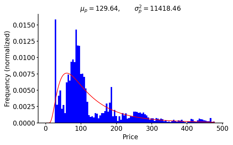
To illustrate this assumption, I have plotted a histogram of the SPDR S&P 500 Trust ETF’s (SPY) prices along with the best-fit log normal distribution (Figure $3$). I used scipy.stats.lognorm.fit to fit the distribution, and again, data is from Yahoo! Finance. We can see that, as a first approximation, the log normal distribution is not completely unreasonable, but it’s certainly not a good model of these data.

Compounded return

Consider Equation $6$ for computing continuously compounded returns. If we take $\log(1 + x)$ of both sides, we get

$\begin{aligned} z_{0:T} &= \log(1 + r_{0:T}) \\ &= \log \left( \prod_{t=1}^T (1 + r_t) \right) \\ &= \sum_{t=1}^T \log (1 + r_t). \end{aligned} \tag{16}$

Furthermore, notice that implicit in each term $r_t$ are the prices $p_t$ and $p_{t-1}$, and that most of these terms will cancel:

$\begin{aligned} z_{0:T} &= \sum_{t=1}^T \log (1 + r_t) \\ &= \sum_{t=1}^T \log\left( \frac{p_t}{p_{t-1}} \right) \\ &= \sum_{t=1}^T \left[ \log p_t - \log p_{t-1} \right] \\ &= \log p_T - \log p_0. \end{aligned} \tag{17}$

So one nice mathematical fact about log returns is that we can compute continuously compounding returns by subtracting the log of the initial price from the log of the final price.

For example, using the data in Figure $1$, AAPL’s total compounded return is approximately $3.14\%$. If we had invested $$100$ in AAPL at the beginning of January $2019$ and held until the end of $2021$, we would now have over $$300$. We can verify that our calculations are consistent, regardless of whether we use Equation $6$ or Equation $17$:

>>> (1 + returns).prod() - 1
3.1448448132962152
>>> np.exp(np.log(closes[-1]) - np.log(closes[0])) - 1
3.1448448132962152

Note that we had to back out the raw return from the log return using the inverse of Equation $11$,

$r_t = \exp(z_t) - 1. \tag{18}$

Clearly, the second calculation is faster, especially if we have a lot of data.

Approximations

A final reason for log returns is that, in addition to their nice mathematical properties, they often approximate raw returns well. This is because

$\log(1 + x) \approx x \tag{19}$

when $x$ is close to zero, and returns are typically close to zero. The easiest way to see this is to note that at the origin, the tangent line $f(x) = x$ approximates $f(x) = \log(1 + x)$ well (Figure $2$, left).

Formally, we can see this using a first-order Taylor approximation of $f(x) = \log(1 + x)$ at a point $a$:

$\begin{aligned} f(x) &\approx f(a) + f^{\prime}(a)(x - a), \\ &\Downarrow \\ \log(1 + x) &\approx \log(1 + a) + \frac{x - a}{1 + a}. \end{aligned} \tag{20}$

So when $a = 0$ at the origin, then $\log(1 + x) \approx x$. This is for the natural logarithm, of course, since otherwise

$f^{\prime}(a) = \frac{1}{\ln(b) (1 + a)} \tag{21}$

where $b$ is the base. So (natural) log returns are a good approximation of raw returns when the raw returns are close to zero.