Multicollinearity

Linearly dependent predictors

In my first post on linear models, we derived the normal equation for linear regression or ordinary least squares (OLS). Let $\mathbf{y}$ be an $N$-vector of targets, and let $\mathbf{X}$ be an $N \times P$ design matrix of predictors. Then the normal equation for the OLS coefficients $\hat{\boldsymbol{\beta}} = [\hat{\beta}_1, \dots, \hat{\beta}_P]^{\top}$ is

$\hat{\boldsymbol{\beta}} = (\mathbf{X}^{\top} \mathbf{X})^{-1} \mathbf{X}^{\top} \mathbf{y}. \tag{1}$

Note that estimating $\hat{\boldsymbol{\beta}}$ depends on the Gram matrix $\mathbf{X}^{\top} \mathbf{X}$ being invertible. Furthermore, the variance of this estimator,

$\mathbb{V}[\hat{\boldsymbol{\beta}} \mid \mathbf{X}] = \sigma^2 (\mathbf{X}^{\top} \mathbf{X})^{-1}, \tag{2}$

also depends on $\mathbf{X}^{\top} \mathbf{X}$ being invertible. Therefore, a key question for OLS is: when is $\boldsymbol{\Sigma} \triangleq \mathbf{X}^{\top} \mathbf{X}$ invertible? $\boldsymbol{\Sigma}$ is invertible if and only if $\mathbf{X}$ is full rank, and $\mathbf{X}$ is full rank when none of its $P$ columns can be represented as linear combinations of any other columns. See A1 for a proof of this claim. (Notice that this immediately implies that $N \geq P$, since the $P$ columns of $\mathbf{X}$ cannot be linearly independent if their size is less than $P$. See my discussion of the linear–dimension inequality in my post on linearly dependence if needed. Thus, OLS requires that there be as many observations as predictors.)

If the predictors of $\mathbf{X}$ are linearly dependent, then we say they are multicollinear, and we call this phenomenon exact multicollinearity. However, in practice, our predictors rarely exhibit exact multicollinearity, as this would mean two predictors are effectively the same. However, multicollinearity can still be a problem without a perfect linear relationship between predictors. First, models can be difficult to interpret since multicollinear predictors can be predictive of the same response. Second, the matrix inversion of $\boldsymbol{\Sigma}$ may be impossible at worst and unstable at best. If the inversion is unstable, the estimated $\hat{\boldsymbol{\beta}}$ can change dramatically given a small change in the input.

Let’s discuss both problems in turn.

Uninterpretible features

The first problem with multicollinearity is that it makes it difficult to disambiguate between the effect of two or more multicollinear predictors. Imagine, for example, that we use a linear model to predict housing prices and that two predictors, $x_1$ and $x_2$, both measure the size of the house. One is the area in square feet, and the other is the area in square meters. Since $x_1$ and $x_2$ are collinear, then $x_1 = K x_2$ for some constant $K$ and therefore:

$\begin{aligned} y &= \beta_0 + \beta_1 x_1 + \beta_2 x_2 + \dots + \beta_P x_P + \varepsilon \\ &= \beta_0 + \overbrace{(\beta_1 K + \beta_2)}^{\beta_{\star}} x_2 + \dots + \beta_P x_P + \varepsilon. \end{aligned} \tag{3}$

Here, there is no unique solution to the normal equation (recall there are $N$ such equations and $P \leq N$). For any choice of $\beta_1$, there is an infinite number of choices for $\beta_2$ through the equation $\beta_{\star} \triangleq \beta_1 K + \beta_2$. Given this fact, it is difficult to properly interpret $\beta_1$ and $\beta_2$ since, in principal, they can be any value. This also has downstream effects. If the variance of $\hat{\boldsymbol{\beta}}$ is high, then it will be harder to reject the null hypothesis.

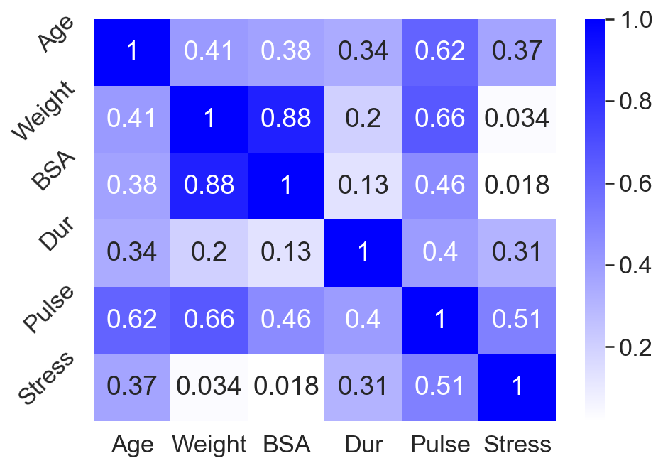
As an example of this behavior, consider predicting blood pressure using the data in A2. The predictors are age (years), weight (kilograms), body-surface area (square meters), duration of hypertension (years), basal pulse (beats per minute), and stress index. Since body-surface area (BSA) and weight are highly correlated (Figure $1$), we hypothesize that these data exhibit multicollinearity. (I’ll discuss a quantitative test for multicollinearity later.)

Figure 1. Correlation matrix for predictors in the blood pressure data set. Weight and BSA are highly correlated.

To see the affects of multicollinearity, I fit OLS to three different subsets of predictors: all predictors, only weight, and only BSA. As we can see in Figure $2$, the OLS coefficients can be tricky to interpret. Based on the coefficients from fitting OLS to all predictors (Figure $2$, left), we might expect BSA to be the most important feature for predicting blood pressure. However, looking at the coefficients for OLS fit to just weight (Figure $2$, middle) and just BSA (Figure $2$, right) complicates the picture. We find that weight is actually more predictive of blood pressure, as measured by the coefficient of determination $R^2$. This is because BSA, weight, and blood pressure are all correlated, but weight is more highly correlated with blood pressure than BSA is. However, when both predictors are included in the model, multicollinearity complicates the analysis.

Figure 2. OLS coefficients and goodness-of-fit ($R^2$) on blood pressure data for (left) all predictors, (middle) just the weight predictor, and (right) just the BSA predictor.

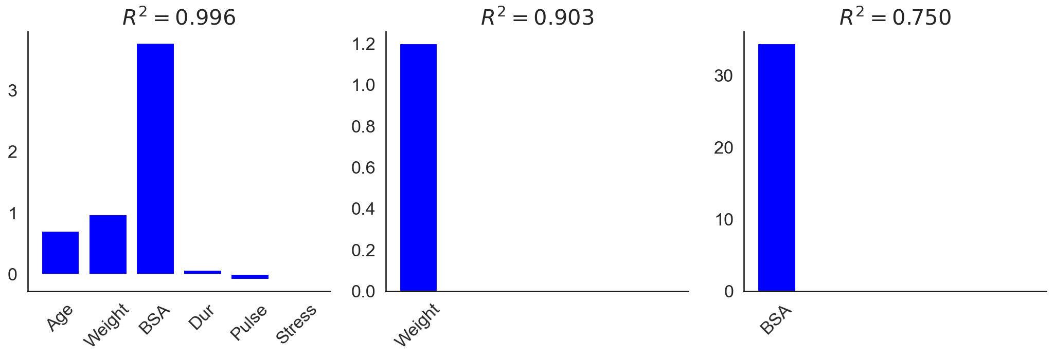
Also notice that the BSA-only model’s coefficient is quite large. My understanding is that extreme values, as well as sign changes, suggest that a data set may suffer from multicollinearity.

Unstable parameter estimates

The second problem of multicollinearity is that our parameter estimates will be algorithmically unstable. To see this, let’s quantify multicollinearity using the condition number of a matrix. In general, a well-conditioned problem is a problem in which a small change in the input $\mathbf{x}$ results in a small change in the output $f(\mathbf{x})$. An ill-conditioned problem is a problem in which a small change in the input $\mathbf{x}$ results in a large change in the output $f(\mathbf{x})$.

The condition number of a matrix $\mathbf{A}$, denoted $\kappa(\mathbf{A})$, is the ratio of its smallest to largest singular values,

$\kappa(\mathbf{A}) \triangleq \frac{\sigma_1(\mathbf{A})}{\sigma_P(\mathbf{A})}, \tag{4}$

where $\sigma_1(\mathbf{A}) \geq \sigma_2(\mathbf{A}) \geq \dots \geq \sigma_P(\mathbf{A})$ are the singular values of $\mathbf{A}$. As we can see, when the smallest singular value $\sigma_P(\mathbf{A})$ is close to zero, the condition number of $\mathbf{A}$ is big.

But what’s the intuition behind this definition? Consider the singular value decomposition (SVD) of a matrix $\mathbf{A}$:

$\mathbf{A} = \mathbf{U}\mathbf{S}\mathbf{V}^{\top}, \tag{5}$

where $\mathbf{U}$ and $\mathbf{V}$ are orthogonal matrices, and $\mathbf{S}$ is a diagonal matrix of singular values:

$\mathbf{S} = \begin{bmatrix} \sigma_1(\mathbf{A}) & & & \\ & \sigma_2(\mathbf{A}) & & \\ & & \ddots & \\ & & & \sigma_P(\mathbf{A}) \\ \end{bmatrix}. \tag{6}$

Then the inverse of $\mathbf{A}$ can be written as

$\mathbf{A}^{-1} = \mathbf{V}\mathbf{S}^{-1}\mathbf{U}^{\top}, \tag{7}$

where, since $\mathbf{S}$ is a diagonal matrix, it’s inverse is just the inverse of its diagonal elements:

$\mathbf{S}^{-1} = \begin{bmatrix} 1/\sigma_1(\mathbf{A}) & & & \\ & 1/\sigma_2(\mathbf{A}) & & \\ & & \ddots & \\ & & & 1/\sigma_P(\mathbf{A}) \\ \end{bmatrix}. \tag{8}$

As we can see, when any singular value of $\mathbf{A}$ is zero, the matrix inverse does not exist. And when any singular value is small, then matrix inversion can be numerically unstable. This is because $1 / \sigma_p(\mathbf{A})$ is sensitive to the value of $\sigma_p(\mathbf{A})$ because we are representing continuous values with discrete machines. For example, a small increase in $\sigma_p(\mathbf{A})$ might result in numerical underflow.

Thus, the size of the singular values matters for both the mathematical existence of the matrix inverse $\mathbf{A}^{-1}$, as well as algorithmic stability of computing that inverse even when it does technically exist, i.e. when no singular value is exactly zero. See (Trefethen & Bau III, 1997) for a thorough discussion of condition numbers and algorithmic stability.

This is why Python libraries such statsmodels will warn us about eigenvalues (square of the singular values) if we fit OLS to data with multicollinearity, e.g.:

import numpy as np
import statsmodels.api as sm

N = 100
X = np.random.normal(size=(N, 1))
X = np.hstack([X, 2*X])
y = np.random.normal(size=N)

ols = sm.OLS(y, sm.add_constant(X))
res = ols.fit()
print(res.summary())

# The smallest eigenvalue is 1.88e-30. This might indicate that there are
# strong multicollinearity problems or that the design matrix is singular.

It’s not necessarily correlation

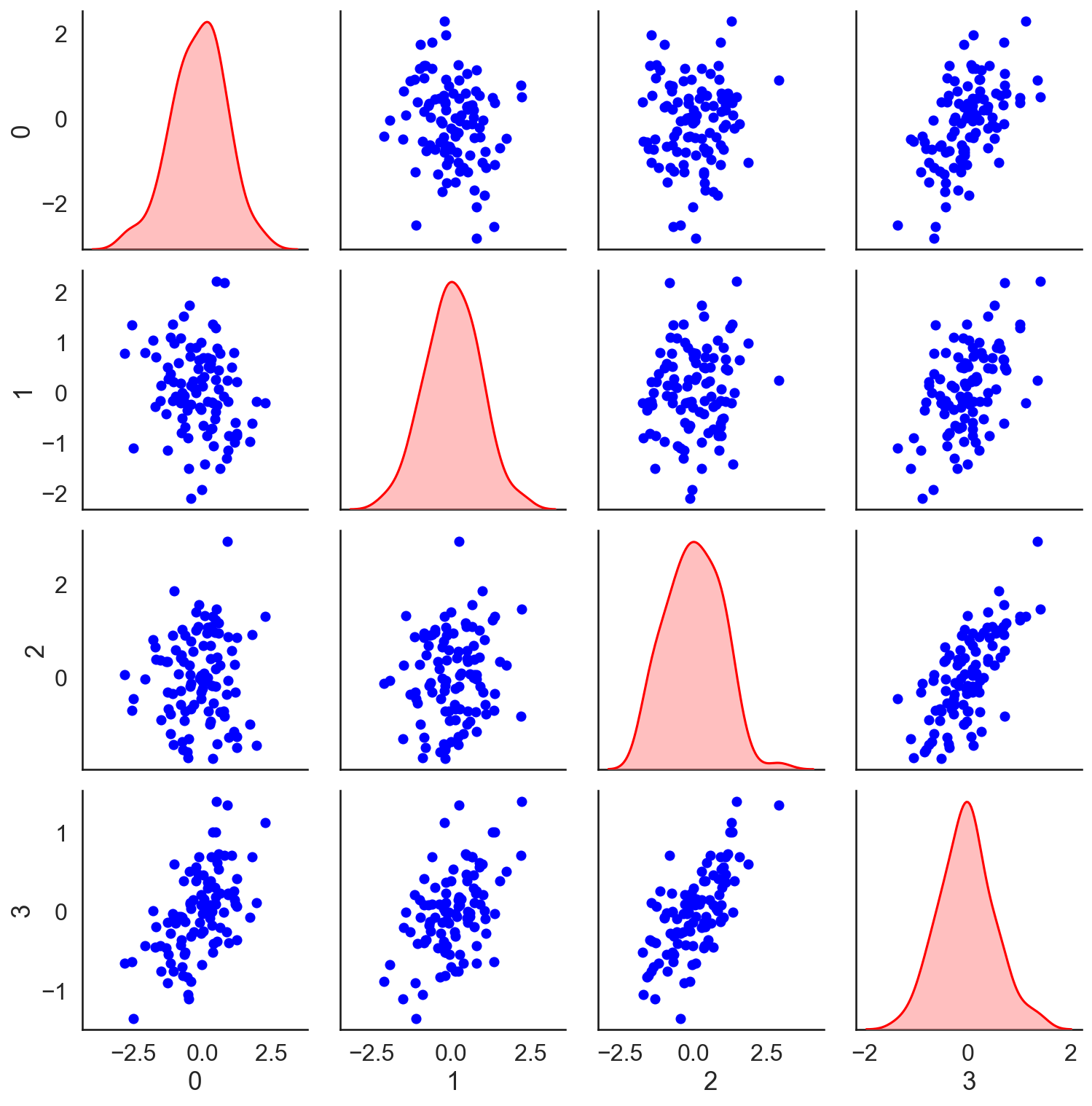
As a caveat, note that multicollinearity is about linear dependence between columns $\mathbf{X}$, which is not the same thing as correlation between the predictors, although it often is. In fact, we can have a set of columns of $\mathbf{X}$ that are multicollinear without significant correlation between predictors. Consider, for example, three i.i.d. Gaussian random vectors and one vector that is the average of the previous three. The vectors are not highly correlated (Figure $3$), but the design matrix has a large condition number. Running this experiment once on my machine, the condition number of the correlation matrix of the first three predictors (the top left block of Figure $3$) is approximately $1.5$. The condition number of all four predictors is approximately $1.3 \times 10^{15}$.

Figure 3. Pairwise relationships of three predictors which are i.i.d. Gaussian and a fourth which is the average of the first three. The design matrix has a large condition number, but the predictors are not highly correlated.

Treatment

Now that we understand multicollinearity and how to detect it, how can we treat the issue? An obvious thing to try would be to just drop a predictor if it is highly correlated with another one. However, this may not be the best approach. As we saw above, it is possible for a set of predictors to exhibit multicollinearity without any two predictors being too highly correlated. Furthermore, all things being equal, we’d probably prefer to use data rather than discard it.

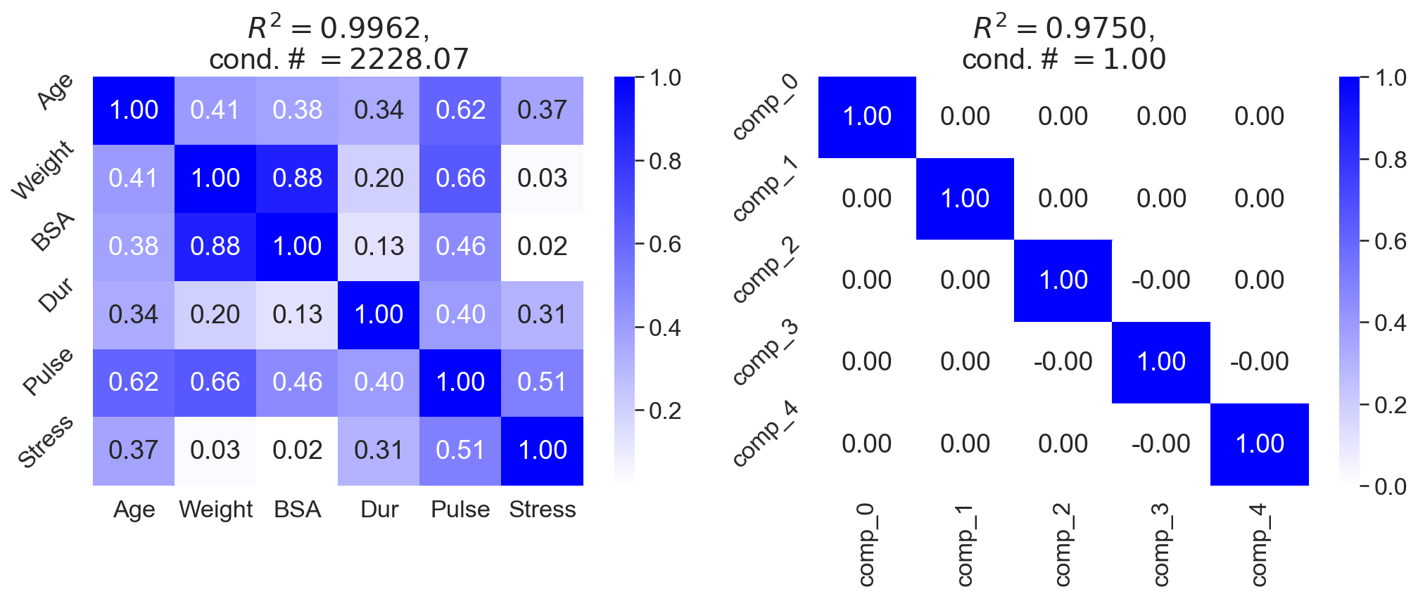
However, one useful treatment is to use dimension reduction. Methods such as partial least squares regression and principal component regression both perform linear dimension reduction on the predictors. For example, I fit OLS to both the blood pressure data (Figure $4$, left) and the latent factors after fitting principal components analysis (PCA) to the blood pressure data (Figure $4$, right). Both approaches have a similar coefficient of determination, but the second approach does not exhibit multicollinearity.

Figure 4. The correlation matrices of the blood pressure data (left) and latent factors from PCA (right).

Another approach to mitigating the affects of multicollinearity is to use ridge regression. Recall that ridge regression introduces Tikhonov regularization or an $\ell_2$-norm penalty to the weights $\boldsymbol{\beta}$. Ridge regression is so-named because the new optimization amounts to adding values along the diagonal (or “ridge”) of the covariance matrix,

$\hat{\boldsymbol{\beta}}_{\textsf{ridge}} = (\alpha \mathbf{I} + \mathbf{X}^{\top} \mathbf{X})^{-1} \mathbf{X}^{\top} \mathbf{y}, \tag{9}$

where $\alpha > 0$ is a hyperparameter. Adding elements to the diagonal of $\boldsymbol{\Sigma}$ ensures that the matrix is full rank, and thus invertible. This is also useful in low-data scenarios, when $P \gt N$.

Conclusion

Multicollinearity is an important challenge when fitting and interpreting linear models. The phenomenon is not necessarily about correlation between predictors, and it is not necessarily an issue for the goodness-of-fit or the quality of the predictions. Rather, multicollinearity is about linear dependence between predictors in the design matrix $\mathbf{X}$, which results in numerical instability when estimating $\boldsymbol{\beta}$ through inverting the Gram matrix $\boldsymbol{\Sigma}$. We can detect multicollinearity by analyzing the singular values of $\mathbf{X}$, and we can mitigate its effects through techniques such as dimension reduction and regularization.

Appendix

A1. Proof that $\mathbf{G} = \mathbf{A}^{\top} \mathbf{A}$ is invertible iff $\mathbf{A}$ is full rank

Any Gram matrix $\mathbf{G} \triangleq \mathbf{A}^{\top} \mathbf{A}$ is uninvertible if and only if the columns of $\mathbf{A}$ are linearly dependent. This is straightforward to prove. First, assume that the columns of $\mathbf{A}$ are linearly dependent. By definition of linear dependence, there exists some vector $\mathbf{x} \neq \mathbf{0}$ such that $\mathbf{Ax} = \mathbf{0}$. It follows immediately that

$\begin{aligned} \mathbf{A} \mathbf{x} &= \mathbf{0} \\ \mathbf{A}^{\top} \mathbf{A} \mathbf{x} &= \mathbf{0} \\ \mathbf{G} \mathbf{x} &= \mathbf{0}. \end{aligned} \tag{A1.1}$

Since $\mathbf{x} \neq \mathbf{0}$ by assumption, $\mathbf{G}$ is uninvertible. The last step is because one definition of an invertible matrix is that the equation $\mathbf{A}\mathbf{x} = \mathbf{0}$ only has the trivial solution $\mathbf{x} = \mathbf{0}$. Now assume that $\mathbf{G}$ is uninvertible. So there exists a vector $\mathbf{x} \neq \mathbf{0}$ such that $\mathbf{Gx} = \mathbf{0}$. Then

$\begin{aligned} \mathbf{G} \mathbf{x} &= \mathbf{0} \\ \mathbf{x}^{\top} \mathbf{G} \mathbf{x} &= \mathbf{0} \\ \lVert \mathbf{Ax} \rVert_2^2 &= \mathbf{0}. \end{aligned} \tag{A1.2}$

Therefore $\mathbf{Ax} = \mathbf{0}$ while $\mathbf{x} \neq \mathbf{0}$. The columns of $\mathbf{A}$ are linearly dependent.

A2. Blood pressure data

These data are taken from here:

Pt  BP   Age  Weight  BSA   Dur  Pulse  Stress
1   105  47   85.4    1.75  5.1  63     33
2   115  49   94.2    2.10  3.8  70     14
3   116  49   95.3    1.98  8.2  72     10
4   117  50   94.7    2.01  5.8  73     99
5   112  51   89.4    1.89  7.0  72     95
6   121  48   99.5    2.25  9.3  71     10
7   121  49   99.8    2.25  2.5  69     42
8   110  47   90.9    1.90  6.2  66     8
9   110  49   89.2    1.83  7.1  69     62
10  114  48   92.7    2.07  5.6  64     35
11  114  47   94.4    2.07  5.3  74     90
12  115  49   94.1    1.98  5.6  71     21
13  114  50   91.6    2.05  10.2 68     47
14  106  45   87.1    1.92  5.6  67     80
15  125  52   101.3   2.19  10.0 76     98
16  114  46   94.5    1.98  7.4  69     95
17  106  46   87.0    1.87  3.6  62     18
18  113  46   94.5    1.90  4.3  70     12
19  110  48   90.5    1.88  9.0  71     99
20  122  56   95.7    2.09  7.0  75     99