Linear Independence, Basis, and the Gram–Schmidt algorithm

Definitions

A collection of one or more $d$-vectors $\mathbf{a}_1, \dots, \mathbf{a}_n$ is called linearly dependent if

$\mathbf{0} = \alpha_1 \mathbf{a}_1 + \dots + \alpha_n \mathbf{a}_n, \tag{1}$

for some scalars $\alpha_1, \dots, \alpha_n$ which are not all zero and where $\mathbf{0}$ is a $d$-vector of zeros. The definition of linear independence is just the opposite notion. A collection of $d$-vectors are linearly independent if the only way to make them equal to the zero-vector is if all the coefficients are zero:

$\mathbf{0} = \alpha_1 \mathbf{a}_1 + \dots + \alpha_n \mathbf{a}_n \quad\iff\quad \alpha_1 = \dots = \alpha_n = 0. \tag{2}$

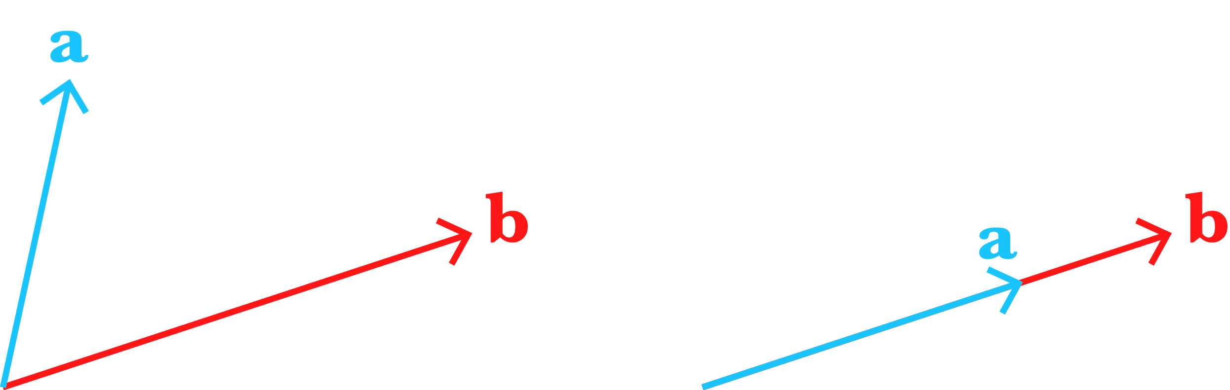
For example, here are two pairs of $2$-vectors that are linearly independent (left) and linearly dependent (right):

$\mathbf{u}_1 = \begin{bmatrix} 1 \\ 0 \end{bmatrix}, \quad \mathbf{u}_2 = \begin{bmatrix} 1 \\ -3 \end{bmatrix}, \qquad\qquad \mathbf{v}_1 = \begin{bmatrix} 1 \\ 2 \end{bmatrix}, \quad \mathbf{v}_2 = \begin{bmatrix} 2 \\ 4 \end{bmatrix}. \tag{3}$

The vectors $\mathbf{v}_1$ and $\mathbf{v}_2$ are dependent since $-2 \mathbf{v}_1 + \mathbf{v}_2 = \mathbf{0}$.

Why do we use the word “dependence” to describe Equation $1$? Since $\alpha_i \neq 0$ for at least one vector for a linearly dependent set, we can rewrite Equation $1$ as

$\mathbf{a}_i = (-\alpha_1/\alpha_i) \mathbf{a}_1 + \dots + (-\alpha_{i-1} / \alpha_i) \mathbf{a}_{i-1} + (-\alpha_{i+1} / \alpha_i) \mathbf{a}_{i+1} + (-\alpha_n/\alpha_i) \mathbf{a}_n. \tag{4}$

In other words, any vector $\mathbf{a}_i$ for which $\alpha_i \neq 0$ can be written as a linear combination of the other vectors in the collection. This is the mathematical formulation for why we call the vectors “dependent.” It’s because we can express the vectors in terms of each other.

Geometric interpretations

Let’s visualize linear dependence and independence. Recall that vector addition $\mathbf{a} + \mathbf{b}$ can be visualized by first drawing the vector $\mathbf{a}$ from the origin and then drawing the vector $\mathbf{b}$ from the head of $\mathbf{a}$. The resulting vector $\mathbf{a} + \mathbf{b}$ is the vector from the origin to head of $\mathbf{b}$ (Figure $1$). Note that we can flip the order, drawing the vector $\mathbf{b}$ and then $\mathbf{a}$ and still arrive at the same location.

Figure 1. Visualization of vector addition $\mathbf{a} + \mathbf{b}$.

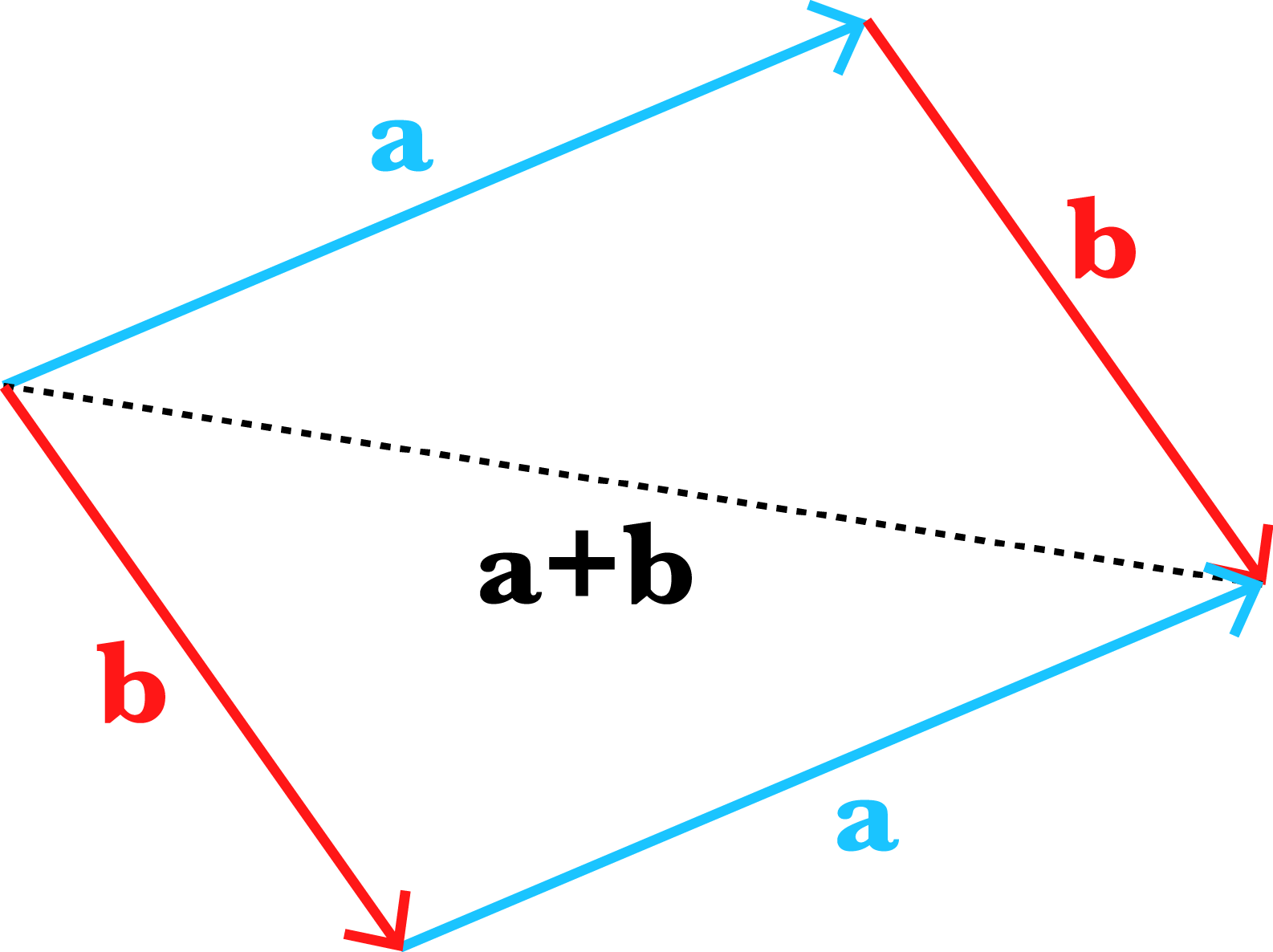
Now what does it mean for two $2$-vectors to be scaled such that they add to $\mathbf{0} = [0, 0]$? It means they must lie on the same line (Figure $2$). Intuitively, if they did not lie on the same line, there would be no way to scale and add the vectors such that the computation ends at the origin $\mathbf{0} = [0, 0]$.

Figure 2. Visualization of two linear independent (left) and dependent (right) vectors in $2$-dimensions.

Notice that if two $2$-vectors are linearly dependent, we can increase the vectors’ size or dimension by adding zeros and still have linearly dependent vectors. For example, the linearly dependent vectors $\mathbf{v}_1$ and $\mathbf{v}_2$ in Equation $3$ are linearly dependent in $3$-dimensions provided we just add zeros:

$\mathbf{v}_1 = \begin{bmatrix} 1 \\ 2 \\ 0 \end{bmatrix}, \quad \mathbf{v}_2 = \begin{bmatrix} 2 \\ 4 \\ 0 \end{bmatrix}. \tag{5}$

Visually, adding zeros in this way is like embedding $2$-vectors on a $2$-dimensional plane into in a $3$-dimensional space.

This starts to suggest what linear dependence in $3$-dimensions might look like. Three linearly dependent $3$-vectors must lie on a plane that goes through the origin (Figure $3$). Again, the visual intuition is that if this were not true, there would be no way to, speaking loosely, get back to the origin $\mathbf{0} = [0,0,0]$ using scaled versions of these vectors. Linear independence in three dimensions is precisely the opposite claim, that the $3$-vectors do not all lie on a plane that passes through the origin.

Figure 3. Visualization of three linear independent (left) and dependent (right) vectors in $3$-dimensions.

Uniqueness

If a vector $\mathbf{v}$ is a linear combination of linearly independent vectors $\mathbf{a}_1, \dots, \mathbf{a}_n$,

$\mathbf{v} = \alpha_1 \mathbf{a}_1 + \dots + \alpha_n \mathbf{a}_n, \tag{6}$

then the coefficients $\alpha_1, \dots, \alpha_n$ are unique. It is easy to prove this. Suppose there are other coefficients $\beta_1, \dots, \beta_n$ such that

$\mathbf{v} = \beta_1 \mathbf{a}_1 + \dots + \beta_n \mathbf{a}_n. \tag{7}$

Then clearly

$\begin{aligned} \mathbf{0} &= \mathbf{v} - \mathbf{v} \\ &= (\alpha_1 \mathbf{a}_1 + \dots + \alpha_n \mathbf{a}_n) - (\beta_1 \mathbf{a}_1 + \dots + \beta_n \mathbf{a}_n) \\ &= (\alpha_1 - \beta_1) \mathbf{a}_1 + \dots + (\alpha_n - \beta_n) \mathbf{a}_n. \end{aligned} \tag{8}$

Since we assumed that the vectors $\mathbf{a}_1, \dots, \mathbf{a}_n$ are linearly independent, then clearly $\alpha_i = \beta_i$ for all $i$.

Dimension and basis

Linear–dimension inequality

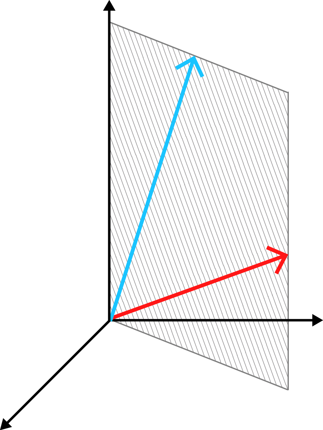
Notice that if we have two $3$-vectors, they could lie on a plane that passes through the origin and still be linearly independent (Figure $4$).

Figure 4. Embedding two linearly independent $2$-vectors into $3$-dimensions.

For example, we can increase the dimension of vectors $\mathbf{u}_1$ and $\mathbf{u}_2$ in Equation $3$ by adding zeros, and the two resultant vectors would still be linearly independent:

$\mathbf{u}_1 = \begin{bmatrix} 1 \\ 0 \\ 0 \end{bmatrix}, \quad \mathbf{u}_2 = \begin{bmatrix} 1 \\ -3 \\ 0 \end{bmatrix}. \tag{9}$

Furthermore, we could even add another vector to this collection such that the new collection is linearly independent, e.g.:

$\mathbf{u}_1 = \begin{bmatrix} 1 \\ 0 \\ 0 \end{bmatrix}, \quad \mathbf{u}_2 = \begin{bmatrix} 1 \\ -3 \\ 0 \end{bmatrix}, \quad \mathbf{u}_3 = \begin{bmatrix} 0 \\ 0 \\ 7 \end{bmatrix}. \tag{10}$

However, we cannot add a new vector to the collection in Equation $10$ and still have a linearly independent set. In general, we cannot have an $n$-sized collection of linearly independent $d$-vectors if $n > d$. However, I think it is an intuitive result. Imagine we had two linearly independent $2$-vectors, such as in Figure $2$. Can you add another vector to the set such that it’s still impossible to scale and add the vectors to return to the origin?

This idea is called the independence–dimension inequality. Formally, if $d$-vectors $\mathbf{a}_1, \dots, \mathbf{a}_n$ are linearly independent, then $n \leq d$. See (Boyd & Vandenberghe, 2018) for a proof. Therefore, a collection of linearly independent $d$-vectors cannot have more than $d$ elements. This immediately implies that any collection of $d+1$ or more $d$-vectors is linearly dependent.

Basis

A basis is a collection of $d$ linearly independent $d$-vectors. Any $d$-vector $\mathbf{v}$ can be written as a linear combination of the vectors in a basis of $d$-vectors:

$\mathbf{v} = \alpha_1 \mathbf{a}_1 + \dots + \alpha_d \mathbf{a}_d. \tag{11}$

The scalars $\alpha_1, \dots, \alpha_d$ are called the coordinates of the basis. As this definition suggests, you are already familiar with this concept. When we use Cartesian coordinates $(x, y)$ to specify the location of an object on the $xy$-plane, those coordinates implicitly rely on the basis vectors $[1, 0]$ and $[0, 1]$:

$\begin{bmatrix} x \\ y \end{bmatrix} = x \begin{bmatrix} 1 \\ 0 \end{bmatrix} + y \begin{bmatrix} 0 \\ 1 \end{bmatrix}. \tag{12}$

Let’s prove that any $d$-vector $\mathbf{v}$ can be represented as a linear combination of a basis of $d$-vectors. Since a basis $\mathbf{a}_1, \dots, \mathbf{a}_d$ is linearly independent, we know that $\alpha_1 = \dots = \alpha_d = 0$ if and only if

$\mathbf{0} = \alpha_1 \mathbf{a}_1 + \dots + \alpha_d \mathbf{a}_d. \tag{13}$

Now consider this basis plus an additional vector $\mathbf{v}$. By the independence–dimension inequality, we know this new collection is linearly dependent. Therefore, it can be written as

$\mathbf{0} = \alpha_1 \mathbf{a}_1 + \dots + \alpha_d \mathbf{a}_d + \nu \mathbf{v}, \tag{14}$

where $\alpha_1, \dots, \alpha_d, \nu$ are not all zero. Then clearly $\nu \neq 0$, otherwise we have a contradiction in our assumption that $\alpha_1 = \dots = \alpha_d = 0$. And if $\nu \neq 0$, we can write the vector $\mathbf{v}$ as a linear combination of the basis vectors:

$\mathbf{v} = (-\alpha_1 / \nu) \mathbf{a}_1 + \dots + (-\alpha_d / \nu) \mathbf{a}_d. \tag{15}$

Furthermore, we proved that if $\mathbf{v}$ is a linear combination of independent vectors, then its coefficients are unique. Combining these two results, we can say: any $d$-vector $\mathbf{v}$ can be uniquely represented as a linear combination of basis vectors $\mathbf{a}_1, \dots, \mathbf{a}_d$.

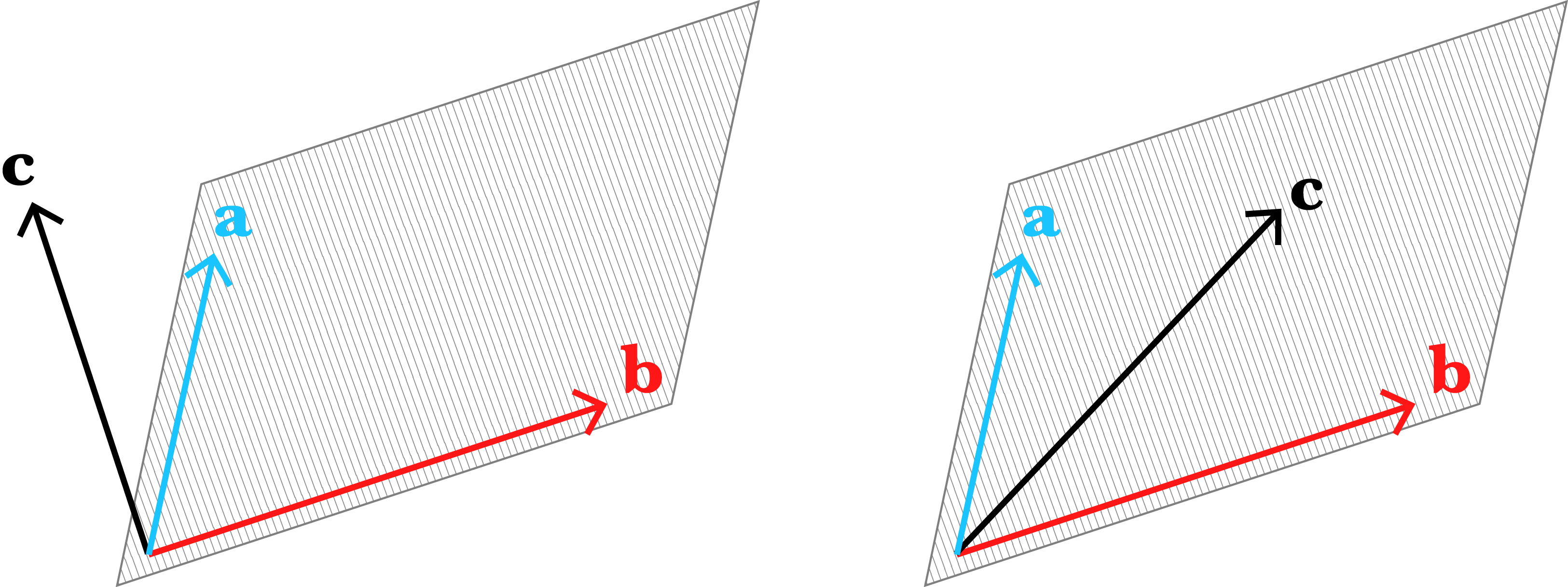
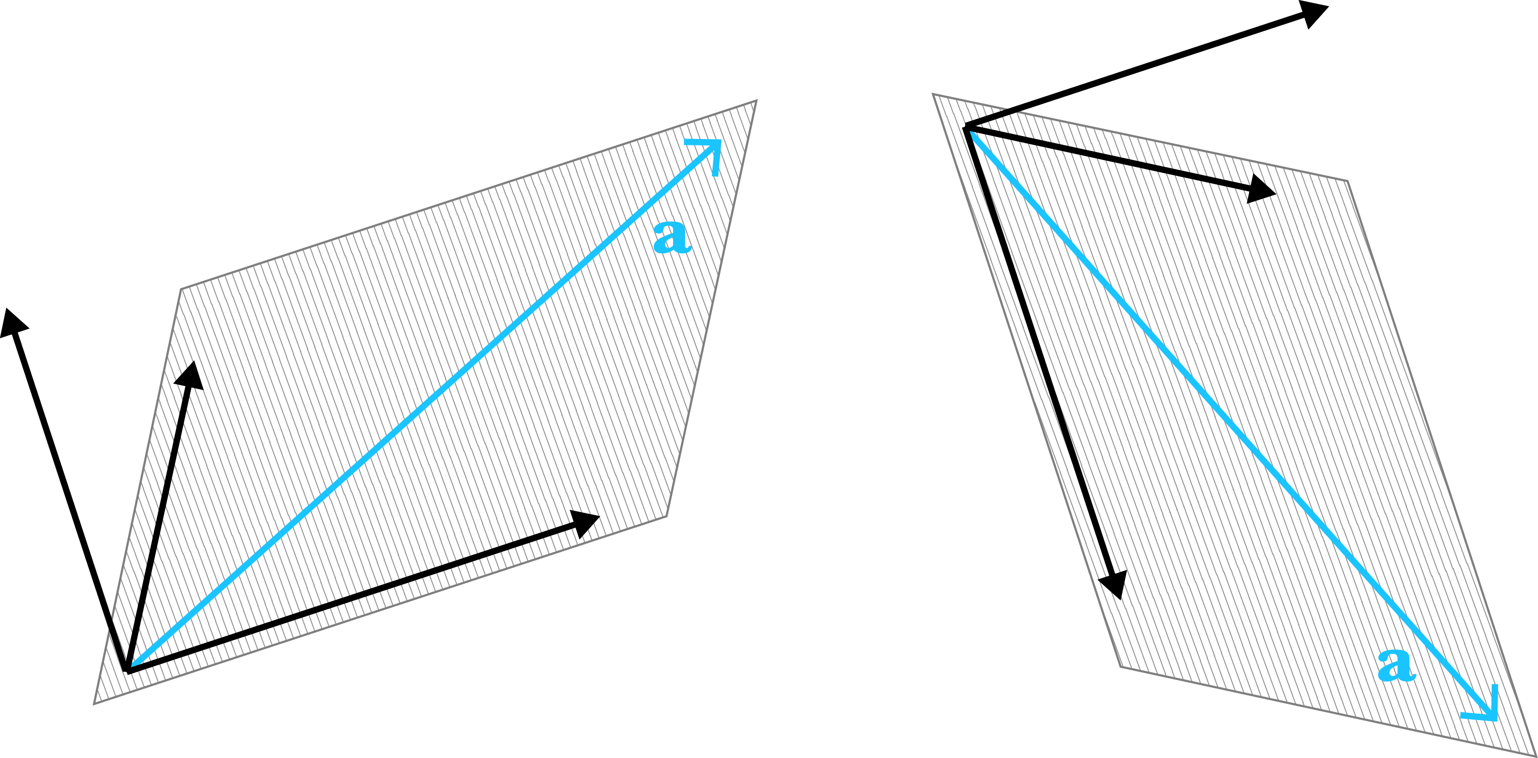
Change of basis

Notice that we can describe the same vector using different bases. I won’t go into this concept in detail, but I think it is quite easy to visualization (Figure $5$). A change of basis is an operation that re-expresses all vectors using a new basis or coordinate system. We’ll see in a bit how the Gram–Schmidt algorithm takes any basis and performs a change-of-basis to an orthonormal basis (discussed next).

Figure 5. A vector $\mathbf{a}$ is represented using two different bases.

Orthogonal and orthonormal vectors

Orthogonality and orthonormality

Two vectors $\mathbf{v}$ and $\mathbf{u}$ are orthogonal if their dot product is zero, i.e.

$\mathbf{v} \cdot \mathbf{u} = 0. \tag{16}$

A collection of vectors $\mathbf{a}_1, \dots, \mathbf{a}_n$ is orthogonal if Equation $16$ holds for any pair of vectors in the collection. A collection $\mathbf{a}_1, \dots, \mathbf{a}_n$ is orthonormal if the collection is both orthogonal and if

$\lVert \mathbf{a}_i \rVert = 1, \qquad i = 1, \dots, n. \tag{17}$

That is, if every vector has unit length. We can express these two conditions as a single condition:

$\mathbf{a}_i \cdot \mathbf{a}_j = \begin{cases} 1 & \text{if $i = j$,} \\ 0 & \text{if $i \neq j$.} \end{cases} \tag{18}$

Orthonormal basis

We can easily prove that orthonormal $d$-vectors are linearly independent. Suppose for some coefficients $\alpha_1, \dots, \alpha_d$

$\alpha_1 \mathbf{a}_1 + \dots + \alpha_d \mathbf{a}_d = \mathbf{0}. \tag{20}$

We can take the dot product of both sides of this equation with any $\mathbf{a}_i$ in the collection to get

$\begin{aligned} \mathbf{0} &= \alpha_1 \mathbf{a}_1 + \dots + \alpha_d \mathbf{a}_d \\ \mathbf{a}_i \cdot \mathbf{0} &= \mathbf{a}_i \cdot (\alpha_1 \mathbf{a}_1 + \dots + \alpha_d \mathbf{a}_d) \\ 0 &= \alpha_1 (\mathbf{a}_i \cdot \mathbf{a}_1) + \dots + \alpha_d (\mathbf{a}_i \cdot \mathbf{a}_d) \\ &\Downarrow \\ 0 &= \alpha_i. \end{aligned} \tag{21}$

The last step holds because of the conditions in Equation $18$. Thus, we have shown that for any $\mathbf{a}_i$ in the collection, its associated coordinate $\alpha_i$ is zero, i.e. orthonormal vectors are linearly independent. Notice that this immediately implies that any $d$-sized collection of orthonormal $d$-vectors is a basis.

Furthermore, notice that if $\mathbf{v}$ is a linear combination of orthonormal vectors, we can use the logic in Equation $21$ to find the coefficients: $\begin{aligned} \mathbf{v} &= \alpha_1 \mathbf{a}_1 + \dots + \alpha_d \mathbf{a}_d \\ \mathbf{a}_i \cdot \mathbf{v} &= \mathbf{a}_i \cdot (\alpha_1 \mathbf{a}_1 + \dots + \alpha_d \mathbf{a}_d) \\ &\Downarrow \\ \mathbf{a}_i \cdot \mathbf{v} &= \alpha_i. \end{aligned} \tag{22}$

The dot product of each vector $\mathbf{a}_i$ in the orthonormal basis with $\mathbf{v}$ equals the associated coefficient.

The standard basis or standard unit vectors are basis of vectors whose coordinates are one-hot vectors, i.e. all zero except for one $1$. For example, the standard basis for $d=2$ is

$\mathbf{e}_1 = \begin{bmatrix} 1 \\ 0 \end{bmatrix}, \quad \mathbf{e}_2 = \begin{bmatrix} 0 \\ 1 \end{bmatrix}. \tag{23}$

Gram–Schmidt algorithm

Imagine we had a collection of $d$-vectors $\mathbf{v}_1, \dots, \mathbf{v}_d$ that formed a basis but that were not necessarily orthonormal. Since orthonormal bases are both convention and easier to work with, a common operation in numerical linear algebra is to convert bases to orthonormal bases. The Gram–Schmidt algorithm is a process for doing that.

Vector projection

Before discussing the Gram–Schmidt algorithm, recall the definition of a vector projection. The vector projection of a vector $\mathbf{a}$ onto a vector $\mathbf{b}$, often denoted $\text{proj}_{\mathbf{b}}(\mathbf{a})$, is

$\text{proj}_{\mathbf{b}}(\mathbf{a}) = \left( \frac{\mathbf{a} \cdot \mathbf{b}}{\lVert \mathbf{b} \rVert} \right) \hat{\mathbf{b}}, \tag{24}$

where $\hat{\mathbf{b}}$ is a unit vector in the direction of $\mathbf{b}$. This definition falls out of a little trigonometry and the definition of the dot product. We know from basic trigonometry that the projection of $\mathbf{a}$ onto $\mathbf{b}$ is $\lVert \mathbf{a} \rVert \cos\theta$, where $\theta$ is the angle between $\mathbf{a}$ and $\mathbf{b}$ (Figure $6$).

Figure 6. Two examples of vector projections of $\mathbf{a}$ onto $\mathbf{b}$. The length of the vector $\mathbf{x}$ is $\lVert \mathbf{a} \rVert \cos \theta$.

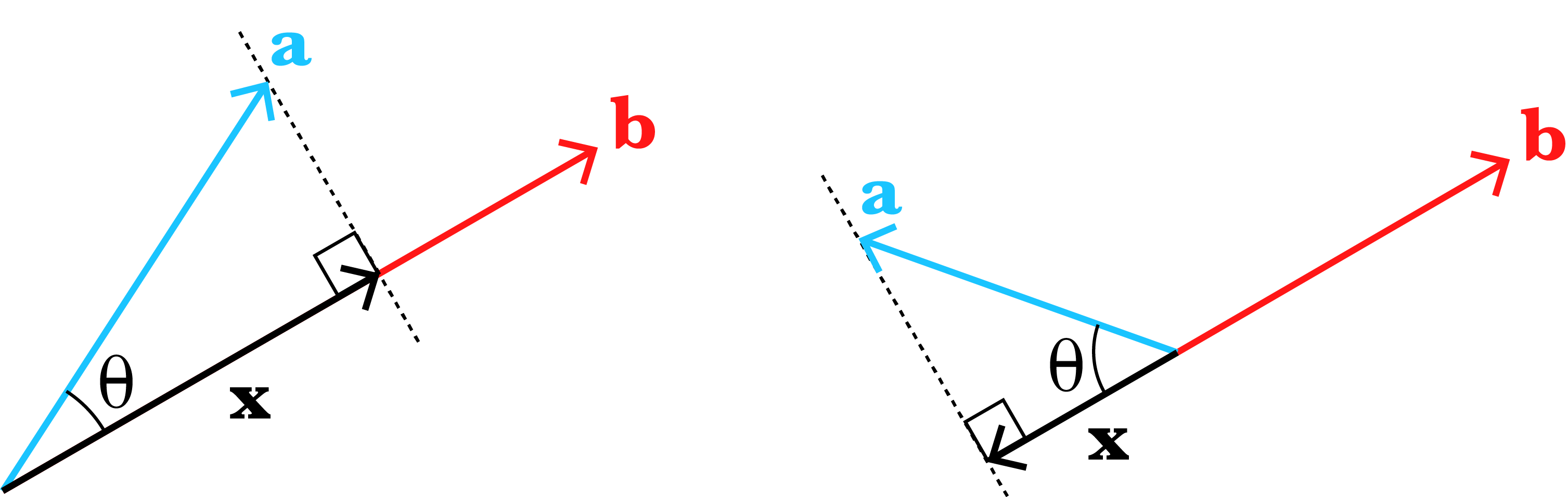
However, if we don’t know $\theta$, we can simply rewrite $\lVert \mathbf{a} \rVert \cos\theta$ using the definition of the dot product,

$\begin{aligned} \mathbf{a} \cdot \mathbf{b} &:= \lVert \mathbf{a} \rVert \lVert \mathbf{b} \rVert \cos\theta \\ &\Downarrow \\ \lVert \mathbf{a} \rVert \cos\theta &= \frac{\mathbf{a} \cdot \mathbf{b}}{\lVert \mathbf{b} \rVert}. \end{aligned} \tag{25}$

This scalar value $(\mathbf{a} \cdot \mathbf{b}) / \lVert \mathbf{b} \rVert$ is the length of the vector $\mathbf{x}$ in Figure $6$, but we must multiply it by a vector that has unit length and points in the direction of $\mathbf{b}$, hence $\hat{\mathbf{b}}$ in Equation $24$.

Algorithm

The Gram–Schmidt algorithm is fairly straightforward. It processes the vectors $\{ \mathbf{v}_1, \dots, \mathbf{v}_d \}$ one at a time while maintaining an invariant: all the previously processed vectors are an orthonormal set. For each vector $\mathbf{v}_i$, it first finds a new vector $\hat{\mathbf{v}}_i$ that is orthogonal to the previously processed vectors. It then normalizes that $\hat{\mathbf{v}}_i$ to a vector we will call $\mathbf{u}_i$. There are plenty of proofs of the correctness of Gram–Schmidt, e.g. (Boyd & Vandenberghe, 2018). In this post, I will just focus on the intuition. I think it’s fairly straightforward to see that Gram–Schmidt should be correct.

Consider the first step of the algorithm. The algorithm processes the vector $\mathbf{v}_1$. Since no other vectors have been processed, $\mathbf{v}_1$ does not need to be changed to be orthogonal to the empty set. The algorithm simply normalizes $\mathbf{v}_1$, i.e. $\mathbf{u}_1 = \mathbf{v}_1 / \lVert \mathbf{v}_1 \rVert$ (Figure $7\text{a}$ and $7\text{b}$).

Figure 7. Gray circles are unit circles. (a) The first vector $\mathbf{v}_1$. (b) $\mathbf{v}_1$ normalized to $\mathbf{u}_1$. (c) A second vector $\mathbf{v}_2$, decomposed into its vector projection onto $\mathbf{v}_1$ and the orthogonal complement of that projection. (d) The new orthogonal vector $\hat{\mathbf{v}}_2$. (e) $\hat{\mathbf{v}}_2$ normalized to $\mathbf{u}_2$.

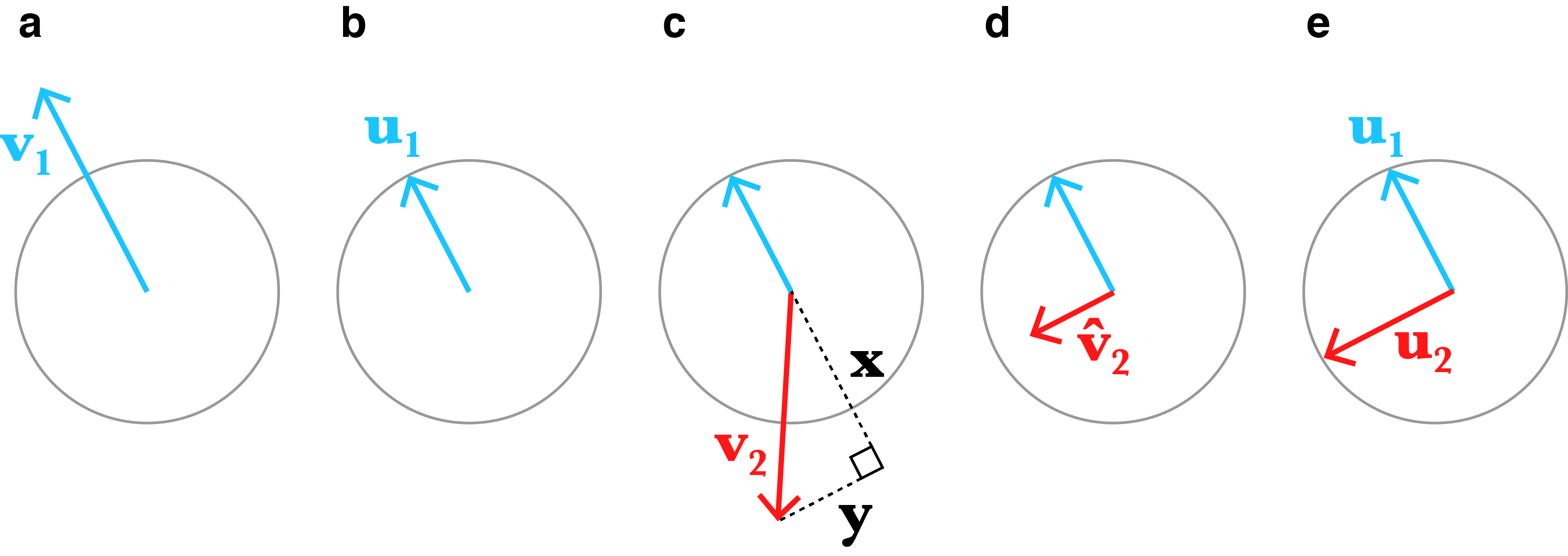
Next, consider the vector $\mathbf{v}_2$, which is not necessarily orthogonal to $\mathbf{u}_1$ (Figure $7\text{c}$). This vector can expressed as the sum of two vectors $\mathbf{x}$ and $\mathbf{y}$, where $\mathbf{x}$ is the projection of $\mathbf{v}_2$ onto $\mathbf{u}_1$ and where $\mathbf{y} = \mathbf{v}_2 - \mathbf{x}$, i.e. it is orthogonal to the vector projection. Therefore, we can find a new vector $\hat{\mathbf{v}}_2$ that is orthogonal to $\mathbf{u}_1$ (Figure $7\text{d}$) as

$\hat{\mathbf{v}}_2 := \mathbf{v}_1 - \text{proj}_{\mathbf{u}_1}(\mathbf{v}_2). \tag{26}$

Finally, we simply normalize $\hat{\mathbf{v}}_2$ to get $\mathbf{u}_2$ (Figure $7\text{e}$). Gram–Schmidt then proceeds by finding a third vector, $\hat{\mathbf{v}}_3$, that is orthogonal to the vectors $\mathbf{u}_1$ and $\mathbf{u}_2$ following the same logic, and so on. In general, the equation for $\hat{\mathbf{v}}_i$ is

$\hat{\mathbf{v}}_i = \mathbf{v}_i - \text{proj}_{\mathbf{u}_1}(\mathbf{v}_i) - \dots - \text{proj}_{\mathbf{u}_{i-1}}(\mathbf{v}_i). \tag{27}$

This is the basic idea of Gram–Schmidt. Besides proving it is correct, there are some other details such as how to handle cases in which the algorithm discovers that $\mathbf{v}_1, \dots, \mathbf{v}_d$ is not a basis. However, I don’t think these add much to the intuition desired here.