Conjugate Gradient Descent

In statistics and optimization, we often want to minimize quadratic functions of the following form,

$f(\mathbf{x}) = \frac{1}{2} \mathbf{x}^{\top} \mathbf{A} \mathbf{x} - \mathbf{b}^{\top} \mathbf{x} + c, \tag{1}$

when $\mathbf{A}$ is a symmetric and positive definite matrix. For example, optimizing a Gaussian log likelihood may reduce to this type of problem. Since $\mathbf{A}$ is symmetric, the gradient is

$\nabla f(\mathbf{x}) = \mathbf{A} \mathbf{x} - \mathbf{b}, \tag{2}$

which implies that the global minimum $\mathbf{x}^{\star}$ is the solution to the equation

$\mathbf{x}^{\star} = \mathbf{A}^{-1} \mathbf{b}. \tag{3}$

See this section on quadratic programming if the derivation above was too fast. An efficient solution to this problem is conjugate gradient descent (CGD), which is gradient descent with a line search that accounts for the positive-definiteness of $\mathbf{A}$. CGD requires no tuning and is typically much faster than gradient descent.

The goal of this post is to understand and implement CGD. There are many excellent presentations of CGD, such as (Shewchuk, 1994). However, I found that many resources focus on deriving various terms rather than the main ideas. The main ideas of CGD are surprisingly simple, and my hope in this post is to make those simple ideas clear.

Gradient descent

Gradient descent is an iterative method. Let $\mathbf{g}_t$ denote the gradient at iteration $t$,

$\mathbf{g}_t \triangleq \nabla f(\mathbf{x}_t) = \mathbf{A}\mathbf{x}_t - \mathbf{b}. \tag{4}$

Gradient descent moves away from the gradient (“downhill”) through the following update rule:

$\mathbf{x}_{t+1} \triangleq \mathbf{x}_t - \alpha_t \mathbf{g}_t. \tag{5}$

In words, given a point $\mathbf{x}_t$ in $N$-dimensional space, we compute the gradient $\mathbf{g}_t$ and then move away from the steepest direction towards the minimum. Given that the size of the gradient has no relationship to how big a step we should to take, we rescale the size of the step with a step size hyperparameter $\alpha_t$. Typically, $\alpha_t$ is constant across iterations, i.e. $\alpha_t = \alpha$.

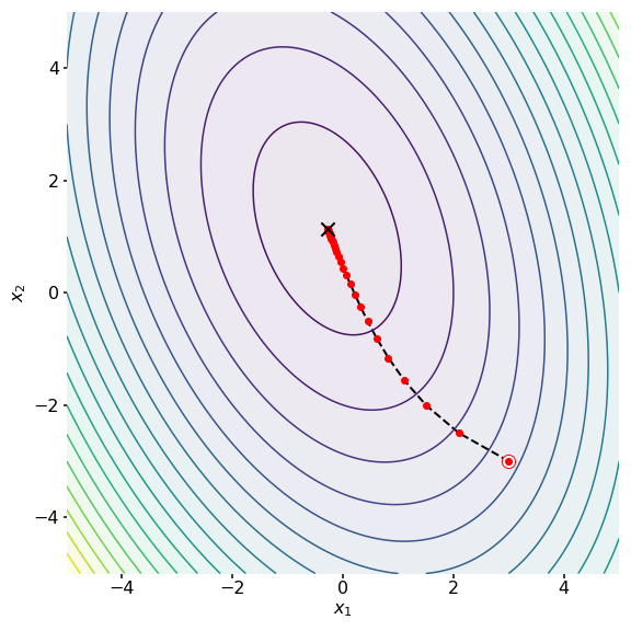
See Figure $1$ for an example of gradient descent in action on a $2$-dimensional problem. We can see that with an appropriate step size, gradient descent moves smoothly towards the global minimum (Figure $1$, black “X”). Throughout this post, I’ll use the values

$\mathbf{A} = \begin{bmatrix} 4 & 1 \\ 1 & 2 \end{bmatrix}, \quad \mathbf{b} = \begin{bmatrix} 0 \\ 2 \end{bmatrix}, \quad c = 10, \tag{6}$

for $\mathbf{A}$, $\mathbf{b}$, and $c$ in Equation $1$.

Figure 1. Gradient descent on the $2$-dimensional quadratic function defined by the values in Equation $6$. The initial point $\mathbf{x}_0$ is the red dot with a white border, and each subsequent step is denoted by a red dot for the location $\mathbf{x}_t$. The global minimum is denoted with a black "X".

In Python, gradient descent can be implement as follows:

def gd(A, b, alpha=1e-3):
    """Run gradient descent with step-size alpha to solve Ax = b.
    """
    dim = A.shape[0]
    x   = np.random.randn(dim)
    xs  = [x]
    while True:
        g = A @ x - b
        x = x - alpha * g
        if np.linalg.norm(x - xs[-1]) < 1e-6:
            break
        xs.append(x)
    return np.array(xs)

This implementation is didactic and obviously avoids many edge-cases for clarity.

Steepest descent

One challenge with gradient descent is that we must pick the step size $\alpha_t$. The gradient tells us in which direction we want to move, but it does not tell us how far we should move. For example, consider the left subplot of Figure $2$. The gradient from the initial point (red dot) suggests that we move along the dashed blue line. However, it may not be obvious how far along this line we should go. Another problem with a fixed step size is that gradient descent can slow down as it approaches the minimum (Figure $1$). In fact, gradient descent took $80$ iterations to converge on this simple problem.

Figure 2. (Left) The initial point $\mathbf{x}_0$ is the red dot with a white border. The black arrow denotes the negative gradient, and the dashed blue line is collinear with this vector. The minimum point along this line is the green dot. (Right) A $3$-dimensional representation of the left subplot. The intersection of the plane implied by the dashed blue line with the quadratic surface is itself a parabola (solid blue line). The initial point $\mathbf{x}_0$ and the minimum of the parabola are denoted with red and green vertical lines, respectively.

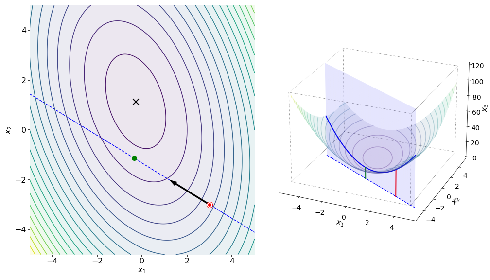
A natural extension to gradient descent is a method sometimes called steepest descent, which automatically computes the optimal step size $\alpha_t$ at each iteration. One way to visualize this is to imagine a line collinear with the gradient (Figure $2$, left, dashed blue line) as being a plane that slices through the quadratic surface. The intersection between this plane and the quadratic surface is a parabola (Figure $2$, right, solid blue line). Intuitively, we want to take a step size $\alpha_t$ that moves us to the minimum of this parabola.

Mathematically, this means that we want to minimize the following:

$\begin{aligned} \alpha^{\star}_t &= \arg\!\min_{\alpha_t} f(\mathbf{x}_t - \alpha \mathbf{g}_t) \\ &= \arg\!\min_{\alpha_t} \left\{ \frac{1}{2} (\mathbf{x}_t - \alpha \mathbf{g}_t)^{\top} \mathbf{A} (\mathbf{x}_t - \alpha \mathbf{g}_t) - \mathbf{b}^{\top} (\mathbf{x}_t - \alpha \mathbf{g}_t) + c \right\} \\ &= \arg\!\min_{\alpha_t} \left\{ \frac{1}{2} ( \mathbf{x}_t^{\top} \mathbf{A} \mathbf{x}_t + \alpha_t^2 \mathbf{g}_t^{\top} \mathbf{A} \mathbf{g}_t - 2 \alpha_t \mathbf{g}_t^{\top} \mathbf{A} \mathbf{x}_t ) - \mathbf{b}^{\top} \mathbf{x}_t + \alpha_t \mathbf{b}^{\top} \mathbf{g}_t + c \right\} \\ &= \arg\!\min_{\alpha_t} \left\{ \frac{1}{2} \alpha_t^2 \mathbf{g}_t^{\top} \mathbf{A} \mathbf{g}_t - \alpha_t \mathbf{g}_t^{\top} \mathbf{A} \mathbf{x}_t + \alpha \mathbf{b}^{\top} \mathbf{g}_t \right\}. \end{aligned} \tag{7}$

To compute the minimizer $\alpha^{\star}_t$, we take the derivative,

$\frac{\partial}{\partial \alpha_t} \left( \frac{1}{2} \alpha_t^2 \mathbf{g}_t^{\top} \mathbf{A} \mathbf{g}_t - \alpha_t \mathbf{g}_t^{\top} \mathbf{A} \mathbf{x}_t + \alpha \mathbf{b}^{\top} \mathbf{g}_t \right) = \alpha_t \mathbf{g}_t^{\top} \mathbf{A} \mathbf{g}_t - \mathbf{g}_t^{\top} \mathbf{A} \mathbf{x}_t + \mathbf{b}^{\top} \mathbf{g}_t, \tag{8}$

and set it equal to zero to solve for $\alpha_t$ (as usual, I am ignoring verifying that $\alpha_t^{\star}$ is not an endpoint or a maximizer):

$\begin{aligned} \alpha_t \mathbf{g}_t^{\top} \mathbf{A} \mathbf{g}_t &= \mathbf{g}_t^{\top} \mathbf{A} \mathbf{x}_t - \mathbf{b}^{\top} \mathbf{g}_t, \\ &\Downarrow \\ \alpha_t^{\star} &= \frac{\mathbf{g}_t^{\top} (\mathbf{A} \mathbf{x}_t - \mathbf{b})}{\mathbf{g}_t^{\top} \mathbf{A} \mathbf{g}_t} \\ &= \frac{\mathbf{g}_t^{\top} \mathbf{g}_t}{\mathbf{g}_t^{\top} \mathbf{A} \mathbf{g}_t}. \end{aligned} \tag{9}$

So the optimal $\alpha_t$ (Equation $9$) leverages the gradient at iteration $t$ and $\mathbf{A}$. Putting it all together, the steepest descent update rules are

$\begin{aligned} \mathbf{g}_t &= \mathbf{A} \mathbf{x}_t - \mathbf{b}, \\ \alpha_t &= \frac{\mathbf{g}_t^{\top} \mathbf{g}_t}{\mathbf{g}_t \mathbf{A} \mathbf{g}_t^{\top}}, \\ \mathbf{x}_{t+1} &= \mathbf{x}_t - \alpha_t \mathbf{g}_t. \end{aligned} \tag{10}$

See Figure $3$ for an example of steepest descent in action on the same $2$-dimensional problem as in Figure $1$. While gradient descent took $80$ iterations, steepest descent took only $21$ iterations. While it is possible that gradient descent could be faster with a bigger step size, we would have to know the optimal step size a priori or tune the algorithm.

Figure 3. Steepest descent on the $2$-dimensional quadratic function defined by the values in Equation $6$. The initial point $\mathbf{x}_0$ is the red dot with a white border, and each subsequent step is denoted by a red dot for the location $\mathbf{x}_t$. The global minimum is denoted with a black "X".

In Python, steepest descent can be implement as follows:

def sd(A, b):
    """Run steepest descent to solve Ax = b.
    """
    dim = A.shape[0]
    x   = np.random.randn(dim)
    xs  = [x]
    while True:
        r     = b - A @ x
        alpha = (r.T @ r) / (r.T @ A @ r)
        x     = x + alpha * r
        if np.linalg.norm(x - xs[-1]) < 1e-6:
            break
        xs.append(x)
    return np.array(xs)

Now consider the following important idea, which will also arise in CGD: in steepest descent, the directions vectors are orthogonal. This is not an accident. Imagine we start at the red dot with a white border in Figure $4$, the initial point $\mathbf{x}_0$. Then imagine that we search along a line that is collinear with the gradient (Figure $4$, blue dashed line). If we compute the gradient at each point along this blue line, the function $f(\mathbf{x}_1)$ is minimized when the gradient is orthogonal to the search line. In Figure $4$, I’ve illustrate this by plotting lines that are collinear with the gradients at various points along the blue line.

Figure 4. The initial point $\mathbf{x}_0$ is the red dot with a white border, and the dashed blue line is collinear with the gradient at $\mathbf{x}_0$. Each gray line is collinear with the gradient at the point at which the gray line intersects the blue line. At the minimum point along the blue line (green dot), the gradient (dashed green line) is perpendicular to the initial direction vector or negative gradient (dashed blue line).

I think this is geometrically intuitive, but we can also prove it from the definition of $\alpha_t$:

$\begin{aligned} \alpha_t &= \frac{\mathbf{g}_t^{\top} \mathbf{g}_t}{\mathbf{g}_t \mathbf{A} \mathbf{g}_t^{\top}}, \\ &\Downarrow \\ \alpha_t \mathbf{g}_t^{\top} \mathbf{A} \mathbf{g}_t &= \mathbf{g}_t^{\top} (\mathbf{A}\mathbf{x}_t - \mathbf{b}), \\ &\Downarrow \\ 0 &= \mathbf{g}_t^{\top} \left[ (\mathbf{A}\mathbf{x}_t - \mathbf{b}) - \alpha_t \mathbf{A} \mathbf{g}_t \right] \\ &= \mathbf{g}_t^{\top} \left[ \mathbf{A} (\mathbf{x}_t - \alpha_t \mathbf{g}_t) - \mathbf{b} \right] \\ &= \mathbf{g}_t^{\top} \left[ \mathbf{A} \mathbf{x}_{t+1} - \mathbf{b} \right] \\ &= \mathbf{g}_t^{\top} \mathbf{g}_{t+1}. \end{aligned} \tag{11}$

This derivation proves that at each iteration $t$, the current gradient $\mathbf{g}_t$ will be orthogonal to the next gradient $\mathbf{g}_{t+1}$. This is precisely why, in Figure $3$, steepest descent repeatedly takes only two directions which are orthogonal to each other, since there are only two dimensions in the problem. Thus, a failure mode of steepest descent is that it can search in the same direction repeatedly. It would be ideal if we could avoid these repeated steps.

The basic idea of conjugate gradient descent is to take steps that are orthogonal with respect to $\mathbf{A}$. This property of orthogonality with respect to a matrix is called “$\mathbf{A}$-orthogonality” or “conjugacy”. (In the phrase “conjugate gradient descent”, “conjugate” modifies “gradient descent”, not the word “gradient”. Thus, CGD is gradient descent with conjugate directions, not conjugate gradients.) Thus, before we can understand conjugate gradient descent, we need to take an aside to understand $\mathbf{A}$-orthogonality. Let’s do that now.

$\mathbf{A}$-orthogonality

Let $\mathbf{A}$ be a symmetric and positive definite matrix. Two vectors $\mathbf{u}$ and $\mathbf{v}$ are $\mathbf{A}$-orthogonal if

$\mathbf{u}^{\top} \mathbf{A} \mathbf{v} = 0, \qquad \mathbf{u} \neq \mathbf{v}. \tag{12}$

The way I think about this is that since $\mathbf{A}$ is symmetric and positive definite, it can be decomposed into a matrix $\mathbf{B}$ such that

$\mathbf{A} = \mathbf{B}^{\top} \mathbf{B}. \tag{13}$

So we can think of Equation $12$ above as

$\mathbf{u}^{\top} \mathbf{B}^{\top} \mathbf{B} \mathbf{v} = (\mathbf{B} \mathbf{u})^{\top} (\mathbf{B} \mathbf{v}) = 0. \tag{14}$

So $\mathbf{A}$-orthogonal means that the two vectors are orthogonal after being mapped by $\mathbf{B}$—loosely speaking, after accounting for the structure of $\mathbf{A}$.

Just as $N$ vectors that are mutually orthogonal form a basis in $\mathbb{R}^N$, $N$ vectors that are $\mathbf{A}$-orthogonal form a basis of $\mathbb{R}^N$. To prove this, let $\mathcal{U} = \{ \mathbf{u}_{n} \}_{n=1}^N$ be a set of mutually $\mathbf{A}$-orthogonal vectors. Now consider the linear combination

$\sum_{n=1}^N \alpha_n \mathbf{u}_n = \mathbf{0}. \tag{15}$

To prove that $\mathcal{U}$ forms a basis, it is sufficient to prove that the set is linearly independent, and to prove that, we must prove that $\alpha_n = 0$ for all $n \in \{1,2,\dots,N\}$. We can do this using the fact that $\mathbf{A}$ is symmetric and positive definite. First, let’s left-multiply Equation $15$ by $\mathbf{u}_m^{\top} \mathbf{A}$ where $\mathbf{u}_m \in \mathcal{U}$:

$\begin{aligned} \mathbf{0} &= \mathbf{u}_m^{\top} \mathbf{A} \left[ \sum_{n=1}^N \alpha_n \mathbf{u}_n \right] \\ &= \sum_{n=1}^N \alpha_n \mathbf{u}_m^{\top} \mathbf{A} \mathbf{u}_n \\ &= \alpha_m \mathbf{u}_m^{\top} \mathbf{A} \mathbf{u}_m. \end{aligned} \tag{16}$

Since $\mathbf{A}$ is positive definite, it must be the case that

$\mathbf{u}_m^{\top} \mathbf{A} \mathbf{u}_m \gt 0. \tag{17}$

This implies that $\alpha_n = 0$ for all $n$, which proves that $\mathcal{U}$ is a linearly independent set, i.e. spans $\mathbb{R}^N$.

Conjugate gradient descent

Let’s return to our problem. How would someone come up with an idea like CGD? Put differently, why would someone think searching in conjugate directions is a good idea? Let $\mathbf{e}_t$ be the error or distance between $\mathbf{x}_t$ and the global minimum $\mathbf{x}^{\star}$ at iteration $t$,

$\mathbf{e}_t \triangleq \mathbf{x}_{t} - \mathbf{x}^{\star}. \tag{18}$

Notice that this error term must be $\mathbf{A}$-orthogonal to the gradient. This falls out of the fact that the gradients are orthogonal:

$\begin{aligned} 0 &= \mathbf{g}_t^{\top} \mathbf{g}_{t+1} \\ &= \mathbf{g}_t^{\top} (\mathbf{A} \mathbf{x}_{t+1} - \mathbf{b}) \\ &= \mathbf{g}_t^{\top} \mathbf{A} (\mathbf{x}_{t+1} - \mathbf{A}^{-1} \mathbf{b}) \\ &= \mathbf{g}_t^{\top} \mathbf{A} \mathbf{e}_{t+1}. \end{aligned} \tag{19}$

In other words, imagine we take the optimal first step using steepest descent (Figure $5$, blue arrow). Then the error between $\mathbf{x}_1$ and $\mathbf{x}^{\star}$ (Figure $5$, green arrow) is conjugate to the initial direction. The blue and green arrows are $\mathbf{A}$-orthogonal by Equation $19$.

Figure 5. The initial point $\mathbf{x}_0$ is the red dot with a white border. The blue vector is the first direction with an optimal step size $\alpha_t$. The difference between $\mathbf{x}_1$ (green dot) and the minimum $\mathbf{x}^{\star}$ (black "X") is the green vector. The blue and green vectors are $\mathbf{A}$-orthogonal by Equation $19$.

What this suggests is that we should search in directions that are $\mathbf{A}$-orthogonal to each other. This is precisely what CGD does.

To see that this approach will work, consider a set of $N$ mutually $\mathbf{A}$-orthogonal or conjugate vectors

$\mathcal{D} = \{\mathbf{d}_1,\dots,\mathbf{d}_N\}. \tag{20}$

Since we proved that these form a basis in $\mathbb{R}^N$, we can express the minimum as a unique linear combination of them

$\mathbf{x}^{\star} = \sum_{n=1}^N \alpha_n \mathbf{d}_n. \tag{21}$

Following the proof of linear independence in the previous section, let’s left-multiply both sides of Equation $21$ by $\mathbf{d}_t^{\top} \mathbf{A}$, where $\mathbf{d}_t \in \mathcal{D}$:

$\mathbf{d}_t^{\top} \mathbf{A} \mathbf{x}^{\star} = \sum_{n=1}^N \alpha_n \mathbf{d}_t^{\top} \mathbf{A} \mathbf{d}_n = \alpha_t \mathbf{d}_t^{\top} \mathbf{A} \mathbf{d}_t. \tag{22}$

The sum disappears because the vectors are mutually conjugate, so

$\mathbf{d}_i^{\top} \mathbf{A} \mathbf{d}_j = 0, \qquad i \neq j. \tag{23}$

And here is the magic. Since $\mathbf{b} = \mathbf{A} \mathbf{x}^{\star}$, we can solve for $\alpha_t$ without using $\mathbf{x}^{\star}$:

$\alpha_t = \frac{\mathbf{d}_t^{\top} \mathbf{b}}{\mathbf{d}_t^{\top} \mathbf{A} \mathbf{d}_t}. \tag{24}$

This is beautiful and surprising to me. What it says is that one way to find the minimum is the following: find $\mathcal{D}$, a set of $N$ mutually conjugate search directions. Next compute each $\alpha_t$. Finally, compute $\mathbf{x}^{\star}$ using Equation $21$. This derivation also makes clear why we need $\mathbf{A}$-orthogonality rather than orthogonality.

This also suggests why we need conjugacy rather than just orthogonality. If $\mathcal{D}$ was a basis formed by $N$ orthogonal directions, then the left-hand side of Equation $22$ would be $\mathbf{d}_t^{\top} \mathbf{x}^{\star}$. We would not be able to eliminate $\mathbf{x}^{\star}$ from the equation.

In Python, this “direct” version of CGD can be implement as follows:

def cgd_direct(A, b):
    """Solve for x in Ax = b directly using an A-orthogonal basis.
    """
    dim = A.shape[0]

    # Run Gram–Schmidt like process to get A-orthogonal basis.
    D = get_conjugate_basis(A)

    # Compute the step size alphas.
    alphas = np.empty(dim)
    for i in range(dim):
        d = D[i]
        alphas[i] = (d @ b) / (d @ A @ d)

    # Directly compute minimum point x_star.
    x_star = np.sum(alphas[:, None] * D, axis=0)
    return x_star

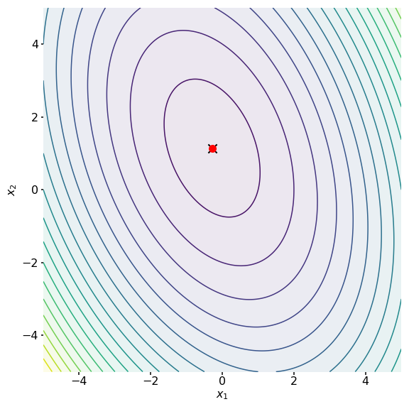
We can see that this correctly computes the minimum point (Figure $6$). Notice that this algorithm does not need an initial point or a step size. It does not even explicitly compute the gradient. It simply constructs an $\mathbf{A}$-orthogonal basis and then expresses the solution $\mathbf{x}^{\star}$ as a linear combination of the basis vectors.

Figure 6. A "direct" approach to CGD finds the minimum point (black "X") without an initial point or a step size.

$\mathbf{A}$-projections

How did we construct a set of mutually $\mathbf{A}$-orthogonal vectors? The basic idea is to run a Gram–Schmidt-like process, ensuring at each step that the newly added vector is $\mathbf{A}$-orthogonal (rather than just orthogonal) to the previous vectors. To understand this approach, let $\mathbf{u}$ and $\mathbf{v}$ be two vectors, and define the $\mathbf{A}$-projection of $\mathbf{v}$ onto $\mathbf{u}$ as

$\text{proj}_{\mathbf{u}}(\mathbf{v}; \mathbf{A}) = \left( \frac{\mathbf{v}^{\top} \mathbf{A} \mathbf{u}}{\mathbf{u}^{\top} \mathbf{A} \mathbf{u}} \right) \mathbf{u}. \tag{25}$

This allows us to construct a new vector that is $\mathbf{A}$-orthogonal to $\mathbf{u}$ by subtracting the $\mathbf{A}$-projection of $\mathbf{v}$ onto $\mathbf{u}$:

$\hat{\mathbf{v}} \triangleq \mathbf{v} - \text{proj}_{\mathbf{u}}(\mathbf{v}; \mathbf{A}). \tag{26}$

We can verify that the resulting vector is $\mathbf{A}$-orthogonal to $\mathbf{u}$:

$\begin{aligned} \mathbf{u}^{\top} \mathbf{A} \hat{\mathbf{v}} &= \mathbf{u}^{\top} \mathbf{A} \left( \mathbf{v} - \left( \frac{\mathbf{v}^{\top} \mathbf{A} \mathbf{u}}{\mathbf{u}^{\top} \mathbf{A} \mathbf{u}} \right) \mathbf{u} \right) \\ &= \mathbf{u}^{\top} \mathbf{A} \mathbf{v} - \cancel{\mathbf{u}^{\top} \mathbf{A} \mathbf{u}} \left( \frac{\mathbf{v}^{\top} \mathbf{A} \mathbf{u}}{\cancel{\mathbf{u}^{\top} \mathbf{A} \mathbf{u}}} \right) \\ &= 0. \end{aligned} \tag{27}$

If why this works does not make sense, I suggest drawing a picture of $\mathbf{A}$-orthogonalization based on my figures on the Gram–Schmidt algorithm in this post. While this is not a proof of correctness for an iterative approach to constructing $\mathcal{D}$, I think it captures the main idea for why it works. A proof would be similar to an induction proof for the correctness of the Gram–Schmidt process.

Here is code to compute an $\mathbf{A}$-orthogonal basis a la the Gram–Schmidt process:

def get_conjugate_basis(A):
    """Run a Gram-Schmidt-like process to get a conjugate basis.
    """
    dim = A.shape[0]
    # Select arbitrary vectors `vs` that form a basis (not necessarily
    # conjugate) in R^dim. Technically, we should verify that `vs` form a basis
    # and handle it if not.
    vs  = np.random.randn(dim, dim)
    v   = vs[0]
    u   = v / np.linalg.norm(v)
    us  = [u]
    for i in range(1, dim):
        v = vs[i]
        for j in range(i):
            v -= proj(A, v, us[j-1])
        u = v / np.linalg.norm(v)
        us.append(u)
    return np.array(us)


def proj(A, v, u):
    """A-project v onto u such that v*A*u is A-orthogonal.
    """
    Au   = A @ u
    beta = (v @ Au) / (u @ Au)
    return beta * u

Notice that if we swapped the function proj for a function that performs the standard projection, we would have the original Gram–Schmidt algorithm. The only difference here is that proj is defined in such a way to ensure that $\mathbf{u}$ and $\mathbf{v}$ are $\mathbf{A}$-orthogonal rather than orthogonal.

An iterative algorithm

While the “direct” method of CGD is conceptually beautiful, it is actually quite expensive if $\mathbf{A}$ is large. Observe that the Gram–Schmidt-like process is repeatedly computing the matrix-vector multiplication $\mathbf{A} \mathbf{u}$. Furthermore, the algorithm runs for $N$ iterations regardless of the structure of the problem. It may be the case that we get close enough to the minimum in fewer than $N$ steps. Ideally, we would early return in this case, but it’s not possible as implemented.

Thus, in practice, CGD does not compute the set $\mathcal{D}$ explicitly beforehand. Instead, it simply starts out in a direction specified by the initial gradient given an initial position, and then constructs each next direction by ensuring it is conjugate to all previous directions. In other words, we simply merge the Gram–Schmidt like process directly into steepest descent, constructing an $\mathbf{A}$-orthogonal basis on the fly. As we’ll see, at each iteration, all but one of the projections are unnecessary, making the algorithm very efficient.

Let’s first look at the basic idea of the iterative approach and then refine it.

Basic idea

Let $\mathbf{r}_t$ denote the residual or negative gradient at iteration $t$:

$\mathbf{r}_t = -\mathbf{g}_t = \mathbf{b} - \mathbf{A}\mathbf{x}_t. \tag{28}$

Let $\mathbf{d}_t$ denote the direction of the step. At each step, we want to construct a new direction vector $\mathbf{d}_{t+1}$ such that it is $\mathbf{A}$-orthogonal to all previous directions.

We initialize with $\mathbf{d}_0 = \mathbf{r}_0$. This just means that we start by following the negative gradient. At iteration $t$, we want the direction $\mathbf{d}_t$ to be conjugate to all the previous directions. Therefore, we subtract the $\mathbf{A}$-projections of all previous directions onto $\mathbf{d}_t$ a la Gram–Schmidt:

$\mathbf{d}_t = \mathbf{r}_t - \sum_{k \lt t} \beta_{tk} \mathbf{d}_k, \tag{29}$

where $\beta_{tk}$ is the conventional notation for the $\mathbf{A}$-projection scalar in Equation $25$,

$\beta_{tk} = \frac{\mathbf{r}_t^{\top} \mathbf{A} \mathbf{d}_k}{\mathbf{d}_k^{\top} \mathbf{A} \mathbf{d}_k}. \tag{30}$

Finally, the step we want to take is in the direction of $\mathbf{d}_t$ with step size $\alpha_t$:

$\mathbf{x}_{t+1} = \mathbf{x}_t + \alpha_t \mathbf{d}_t. \tag{31}$

The optimal $\alpha_t$ is no longer Equation $24$. Instead, we minimize $f(\mathbf{x}_t + \alpha_t \mathbf{d}_t)$ to get:

$\alpha_t = \frac{\mathbf{r}_t^{\top} \mathbf{d}_t}{\mathbf{d}_t^{\top} \mathbf{A} \mathbf{d}_t}. \tag{32}$

I’ll omit this calculation, since we have already done a similar calculation in Equation $7$. Notice that nothing we have done so far should be too surprising. We have just decided that our initial direction vector will be the first residual, and that each subsequent direction will be constructed on the fly from the next residual by subtracting out all $\mathbf{A}$-projections of the residual onto the previous direction vectors. This is essentially a Gram–Schmidt process with $\mathbf{A}$-projections merged into an iterative steepest descent algorithm.

In Python, this iterative version of CGD can be implement as follows:

def cgd_iter(A, b):
    """Run inefficient conjugate gradient descent to solve x in Ax = b.
    """
    dim = A.shape[0]
    x   = np.random.randn(dim)
    xs  = [x]
    ds  = []
        
    for i in range(dim):
        
        # Compute next search direction.
        r = b - A @ x
        
        # Remove previous search directions.
        projs = 0
        for k in range(i):
            d_k     = ds[k-1]
            beta_k  = (r @ A @ d_k) / (d_k @ A @ d_k)
            projs  += beta_k * d_k
        d = r - projs
        
        # Take step.
        alpha = (r @ d) / (d @ A @ d)
        x = x + alpha * d
    
        xs.append(x)
        ds.append(d)

    return np.array(xs)

At each step, we compute the negative gradient $\mathbf{r}_t$ and then subtract out all the previously computed conjugate directions. What is left is a direction $\mathbf{d}_t$ that is conjugate to all the previous directions so far. See Figure $7$ for this version of CGD on our running example.

Figure 7. Conjugate gradient descent on the $2$-dimensional quadratic function defined by the values in Equation $6$. The initial point $\mathbf{x}_0$ is the red dot with a white border, and each subsequent step is denoted by a red dot for the location $\mathbf{x}_t$. The global minimum is denoted with a black "X". The second direction vector is $\mathbf{A}$-orthogonal to the first direction vector, which is just the residual or negative gradient at the initial point.

However, the algorithm above is still not the iterative CGD typically used in practice. This is because we can make the algorithm far more efficient. Let’s look at two optimizations.

Eliminating matrix-vector multiplications

First, observe that there is a recursive relationship between the residuals (and gradients):

$\mathbf{r}_{t+1} = \mathbf{r}_t - \alpha_t \mathbf{A} \mathbf{d}_t. \tag{33}$

This falls out of the update step for the position vector (Equation $31$). First, left-multiply the update step by $\mathbf{A}$ and then subtract each side from $\mathbf{b} = \mathbf{b}$

$\begin{aligned} \mathbf{x}_{t+1} &= \mathbf{x}_t + \alpha_t \mathbf{d}_t, \\ &\Downarrow \\ \mathbf{A} \mathbf{x}_{t+1} &= \mathbf{A} \mathbf{x}_t + \alpha_t \mathbf{A} \mathbf{d}_t, \\ &\Downarrow \\ \mathbf{b} - \mathbf{A} \mathbf{x}_{t+1} &= \mathbf{b} - (\mathbf{A} \mathbf{x}_t + \alpha_t \mathbf{A} \mathbf{d}_t) \\ \mathbf{r}_{t+1} &= \mathbf{r}_t - \alpha_t \mathbf{A} \mathbf{d}_t. \end{aligned} \tag{34}$

Alternatively, we could have subtracted $\mathbf{b}$ from each side to get

$\mathbf{g}_{t+1} = \mathbf{g}_t + \alpha_t \mathbf{A} \mathbf{d}_t \tag{35}$

This is useful because it means that at each iteration, we do not have to compute

$\mathbf{r}_{t+1} = \mathbf{b} - \mathbf{A}\mathbf{x}_{t+1}. \tag{36}$

Instead, after computing $\mathbf{A}\mathbf{d}_t$ to get $\alpha_t$, we can simply subtract these from the current value of $\mathbf{r}_t$ to get the next residual. This eliminates an unnecessary matrix-vector multiplication. (Steepest descent is typically optimized using an equation similar to Equation $35$ to ensure that only one matrix-vector multiplication, $\mathbf{A} \mathbf{g}_t$, is used per iteration.)

Eliminating projections

The second refinement is avoiding most of the steps in $\mathbf{A}$-orthogonalization. In particular, we can prove that

$\beta_{tk} = 0, \quad \forall k \lt t-1. \tag{37}$

In other words, at each iteration, we simply compute a single coefficient $\beta$ using the previous data. There is no need for an inner for-loop or to keep a history of previous directions. In my mind, Equation $37$ is probably the least intuitive aspect of CGD. However, the proof is not that tricky and is instructive for why CGD is so efficient.

First, we need two facts about CGD, two lemmas. The first lemma is that the gradient at iteration $t$ is orthogonal to all the previous search directions, that

$\mathbf{g}_t^{\top} \mathbf{d}_k = 0, \quad \forall k \lt t. \tag{38}$

This is not too surprising if you think about it. We start with an initial gradient, which we follow downhill. We’ve carefully constructed $\alpha_t$ to find the minimum point along the line that is collinear with this gradient, and it makes sense that this minimum point is when the next gradient is orthogonal to the current search direction (Figure $4$ again). However, why is the current search direction orthogonal to all previous gradients? This falls out of the recursive relationship between gradients (Equation $35$). Since the difference between two successive gradients is proportional to $\mathbf{A}\mathbf{d}_t$, then the term $\mathbf{d}_{k}\mathbf{A}\mathbf{d}_t$ is zero for all $k \lt t$. So we can easily use induction to prove Equation $38$ must hold. See A1 for a proof.

We needed the first lemma to prove the second lemma, which that each residual is orthogonal to the previous residuals, that

$\mathbf{r}_{t}^{\top} \mathbf{r}_k = 0, \quad \forall k \lt t. \tag{39}$

This immediately follows out of the definition of $\mathbf{d}_t$ and the previous lemma (see A2).

Finally, we needed the second lemma to prove the main result. Recall the definition of $\beta_{tk}$:

$\beta_{tk} = \frac{\mathbf{r}_t^{\top} \mathbf{A} \mathbf{d}_k}{\mathbf{d}_k^{\top} \mathbf{A} \mathbf{d}_k}. \tag{40}$

We want to prove that $\beta_{tk} = 0$ when $k \lt t-1$. To do this, we will prove that the numerator is zero under the same conditions, that

$\mathbf{r}_t^{\top} \mathbf{A} \mathbf{d}_k = 0, \qquad k \lt t-1. \tag{41}$

To see this, let’s take the dot product of $\mathbf{r}_t$ with Equation $33$ at iteration $k$:

$\mathbf{r}_t^{\top} \mathbf{r}_{k+1} = \mathbf{r}_t^{\top} \mathbf{r}_k - \alpha_k \mathbf{r}_t^{\top} \mathbf{A} \mathbf{d}_k. \tag{42}$

This allows us to write the numerator of $\beta_{tk}$ as

$\mathbf{r}_t^{\top} \mathbf{A} \mathbf{d}_k = \frac{\mathbf{r}_t^{\top} \mathbf{r}_k - \mathbf{r}_t^{\top} \mathbf{r}_{k+1}}{\alpha_k}. \tag{43}$

When $k \lt t-1$, both dot products between residuals on the right-hand side are zero, meaning that $\beta_{tk}$ is zero. Finally, when $k = t-1$, the numerator of $\beta_{tk}$ is

$\mathbf{r}_t^{\top} \mathbf{A} \mathbf{d}_k = -\frac{1}{\alpha_{t-1}} \mathbf{r}_t^{\top} \mathbf{r}_t. \tag{44}$

So $\beta_{tk} = 0$ when $k \lt t-1$. The only search direction we need to $\mathbf{A}$-orthogonalize w.r.t. is the previous one (when $k = t-1$)! As if by magic, all but one of the terms in the Gram–Schmidt-like $\mathbf{A}$-orthogonalization disappear. We no longer need to keep around a history of the previous search directions or to $\mathbf{A}$-orthogonalize the current search direction with any other search direction except the previous one. As I mentioned above, this is probably the least intuitive aspect of CGD, but it simply falls out of the recursive nature of the updates. It’s a bit tricky to summarize at a high level, and I suggest going through the induction proves in the appendices if you are unconvinced.

Since we have proven that we only need to compute a single $\beta$ coefficient at iteration $t$, let’s denote it with $\beta_{t-1}$ instead of $\beta_{t,t-1}$. This gives us

$\mathbf{d}_t = \mathbf{r}_t - \beta_{t-1} \mathbf{d}_{t-1}. \tag{45}$

We can show that $\beta_t$ can be simplified as

$\beta_{t-1} = -\frac{\mathbf{r}_{t}^{\top} \mathbf{r}_{t}}{\mathbf{r}_{t-1}^{\top} \mathbf{r}_{t-1}}. \tag{46}$

This isn’t obvious, but I don’t think it adds much to include the derivation in the main text. See A3 for details. Finally—and this is the final “finally”—let’s redefine $\beta_{t-1}$ as the negative of Equation $46$. Then the final update rule is:

$\mathbf{d}_t = \mathbf{r}_t + \beta_{t-1} \mathbf{d}_{t-1}, \qquad \beta_{t-1} = \frac{\mathbf{r}_{t}^{\top} \mathbf{r}_{t}}{\mathbf{r}_{t-1}^{\top} \mathbf{r}_{t-1}}. \tag{47}$

Putting it all together, conjugate gradient descent is

$\begin{aligned} \textbf{initialize:} & \\ \mathbf{r}_0 &= \mathbf{b} - \mathbf{A} \mathbf{x}_0 && \text{(compute residual from initial position)} \\ \mathbf{d}_0 &= \mathbf{r}_0 && \text{(set initial direction to negative gradient)} \\ \textbf{repeat:} & \\ \alpha_t &= \frac{\mathbf{r}_t^{\top} \mathbf{d}_t}{\mathbf{d}_t^{\top} \mathbf{A} \mathbf{d}_t} && \text{(compute optimal step size)} \\ \mathbf{x}_{t+1} &= \mathbf{x}_{t} + \alpha_t \mathbf{d}_t && \text{(take optimal step)} \\ \mathbf{r}_{t+1} &= \mathbf{r}_{t} - \alpha_t \mathbf{A} \mathbf{d}_t && \text{(efficiently update residual)} \\ \beta_t &= \frac{\mathbf{r}_{t+1}^{\top} \mathbf{r}_{t+1}}{\mathbf{r}_t^{\top} \mathbf{r}_t} && \text{(compute $\mathbf{A}$-projection coefficient)} \\ \mathbf{d}_{t+1} &= \mathbf{r}_{t+1} + \beta_t \mathbf{d}_t && \text{($\mathbf{A}$-orthogonalize next search direction)} \end{aligned}$

Note that we could early return whenever the residual $\mathbf{r}_t$ is small, since it quantifies how good of an estimate $\mathbf{x}_t$ is of the true minimum $\mathbf{x}^{\star}$.

In Python, conjugate gradient descent can be implemented as follows:

def cgd(A, b):
    """Run conjugate gradient descent to solve x in Ax = b.
    """
    dim  = A.shape[0]
    x    = np.random.randn(dim)
    r    = b - A @ x
    d    = r
    rr   = r @ r
    xs   = [x]
        
    for i in range(1, dim):

        # The only matrix-vector multiplication per iteration!
        Ad     = A @ d
        alpha  = rr / (d @ Ad)
        x      = x + alpha * d
        r      = r - alpha * Ad
        rr_new = r @ r
        beta   = rr_new / rr
        d      = r + beta * d
        rr     = rr_new

        xs.append(x)

    return np.array(xs)

While this code may look complex, observe that there is only a single matrix-vector multiplication $\mathbf{A} \mathbf{d}_t$ per iteration. All the other operations are scalar and vector operations. If $\mathbf{A}$ is large, this results in an algorithm that is significantly more efficient than all the other approaches in this post. And ignoring issues related to numerical precision, we are guaranteed to converge in at most $N$ iterations.

Conclusion

Conjugate gradient descent is a beautiful algorithm. The big idea, to construct the minimum point from a basis of conjugate vectors, is simple and easy to prove. An iterative algorithm that constructs this conjugate basis on the fly is efficient because we can prove that the next direction vector is already conjugate to all the previous search directions except for the current one. The final implementation relies on only a single matrix-vector multiplication. If this matrix is large, then CGD is significantly faster than gradient descent or steepest descent.

Acknowledgements

I thank Patryk Guba for correcting a few mistakes in figures and text.

Appendix

A1. Proof of orthogonality of gradients and search directions

Let’s prove

$\mathbf{g}_t^{\top} \mathbf{d}_k = 0, \qquad \forall k \lt t. \tag{A1.1}$

The base case, iteration $t = 0$, is

$\mathbf{g}_1^{\top} \mathbf{d}_0 = 0. \tag{A1.2}$

We can actually prove a stronger claim, that

$\mathbf{g}_{t+1}^{\top} \mathbf{d}_t = 0. \tag{A1.3}$

As before (Equation $11$), this simply falls out of the definition of $\alpha_t$:

$\begin{aligned} \alpha_t &= \frac{\mathbf{r}_t^{\top} \mathbf{d}_t}{\mathbf{d}_t^{\top} \mathbf{A} \mathbf{d}_t} \\ \alpha_t \mathbf{d}_t^{\top} \mathbf{A} \mathbf{d}_t &= \mathbf{r}_t^{\top} \mathbf{d}_t \\ &\Downarrow \\ 0 &= \mathbf{d}_t^{\top} \left[ \mathbf{r}_t - \alpha_t \mathbf{A} \mathbf{d}_t \right] \\ &= \mathbf{d}_t^{\top} \mathbf{r}_{t+1} \\ &= \mathbf{d}_t^{\top} \mathbf{g}_{t+1}. \end{aligned} \tag{A1.4}$

And as before, this is intuitive. Since we have a picked a step size $\alpha_t$ that puts us at the bottom of the parabola described by the intersection of the line-search plane and the quadratic surface (Figure $2$, right), then the next gradient is orthogonal to the previous line search (Figure $4$).

Now for the induction step. Assume that the claim holds at iteration $t$:

$\mathbf{g}_t^{\top} \mathbf{d}_k = 0, \qquad \forall k \lt t. \tag{A1.5}$

We want to prove that, at iteration $t+1$,

$\mathbf{g}_{t+1}^{\top} \mathbf{d}_k = 0, \qquad \forall k \lt t+1. \tag{A1.6}$

In other words, we’re proving that at each subsequent iteration, all new gradients are still orthogonal to $\mathbf{d}_k$. Let’s left-multiply both sides of Equation $35$ by $\mathbf{d}_k$:

$\begin{aligned} \mathbf{d}_k^{\top} \mathbf{g}_{t+1} &= \mathbf{d}_k^{\top} \left( \mathbf{g}_t + \alpha_t \mathbf{A} \mathbf{d}_t \right) \\ &= \mathbf{d}_k^{\top} \mathbf{g}_t + \alpha_t \mathbf{d}_k^{\top} \mathbf{A} \mathbf{d}_t. \end{aligned} \tag{A1.7}$

The left term must be zero because of the induction hypothesis and the right term must be zero because of $\mathbf{A}$-orthogonality. Thus, we have proven that each gradient $\mathbf{g}_t$ is orthogonal to all the previous search directions so far.

A2. Proof of orthogonality of gradients

Let’s prove

$\mathbf{g}_t^{\top} \mathbf{g}_k = 0, \qquad \forall k \lt t. \tag{A2.1}$

(If this holds for the gradients, it holds for the residuals.) This immediately follows from the lemma in A1 and the definition of $\mathbf{d}_t$:

$\begin{aligned} \mathbf{g}_t^{\top} \mathbf{g}_k &= \mathbf{g}_t^{\top} (\mathbf{d}_k - \sum_{j \lt k} \beta_{kj} \mathbf{d}_j) \\ &= \mathbf{g}_t^{\top} \mathbf{d}_k - \sum_{j \lt k} \beta_{kj} \mathbf{g}_t^{\top} \mathbf{d}_j \\ &= 0. \end{aligned} \tag{A2.2}$

So the gradient at iteration $t$ is orthogonal to all the previous gradients, since these are linear functions of the previous search directions.

A3. Simplification of $\beta_{t-1}$

Recall the definition of $\beta_{tk}$:

$\beta_{tk} = \frac{\mathbf{r}_t^{\top} \mathbf{A} \mathbf{d}_k}{\mathbf{d}_k^{\top} \mathbf{A} \mathbf{d}_k}. \tag{A3.1}$

We have proven that $\beta_{tk} = 0$ except when $k = t-1$. We want to show that when $k = t-1$, the following simplification is true:

$\beta_{t-1} = -\frac{\mathbf{r}_{t}^{\top} \mathbf{r}_{t}}{\mathbf{r}_{t-1}^{\top} \mathbf{r}_{t-1}}. \tag{A3.2}$

We know that the numerator can be written as

$-\frac{1}{\alpha_{t-1}} \mathbf{r}_t^{\top} \mathbf{r}_t, \tag{A3.3}$

when $k = t-1$. By Equation $45$, the denominator can be written as

$\begin{aligned} \mathbf{d}_k \mathbf{A} \mathbf{d}_k &= (\mathbf{r}_k - \beta_{k-1} \mathbf{d}_{k-1})^{\top} \mathbf{A} \mathbf{d}_k \\ &= \mathbf{r}_k^{\top} \mathbf{A} \mathbf{d}_k - \beta_{k-1} \mathbf{d}_{k-1}^{\top} \mathbf{A} \mathbf{d}_k \\ &= \mathbf{r}_k^{\top} \mathbf{A} \mathbf{d}_k. \end{aligned} \tag{A3.4}$

And by the recursive relationship between residuals (Equation $33$), we rewrite the last line of Equation $\text{A3.4}$ as

$\begin{aligned} \mathbf{A} \mathbf{d}_k &= -\frac{\mathbf{r}_{k+1} - \mathbf{r}_k}{\alpha_k}, \\ &\Downarrow \\ \mathbf{r}_{k}^{\top} \mathbf{A}\mathbf{d}_k &= -\mathbf{r}_{k}^{\top} \left( \frac{\mathbf{r}_{k+1} - \mathbf{r}_k}{\alpha_k} \right) \\ &= -\frac{1}{\alpha_k} \left( \mathbf{r}_{k}^{\top} \mathbf{r}_{k+1} - \mathbf{r}_{k}^{\top} \mathbf{r}_{k} \right) \\ &= \frac{1}{\alpha_k} \mathbf{r}_{k}^{\top} \mathbf{r}_{k}. \end{aligned} \tag{A3.5}$

Putting it all together and plugging $k = t-1$ into Equation $\text{A3.5}$, we get:

$\begin{aligned} \beta_{t-1} &= \left( -\frac{1}{\alpha_{t-1}} \mathbf{r}_t^{\top} \mathbf{r}_t \right) \bigg/ \left( \frac{1}{\alpha_{t-1}} \mathbf{r}_{t-1}^{\top} \mathbf{r}_{t-1} \right) \\ &= -\frac{\mathbf{r}_{t}^{\top} \mathbf{r}_{t}}{\mathbf{r}_{t-1}^{\top} \mathbf{r}_{t-1}}. \end{aligned} \tag{A3.6}$