Understanding Positive Definite Matrices

A real-valued matrix $\mathbf{A}$ is positive definite if, for every real-valued vector $\mathbf{x}$,

$\mathbf{x}^{\top} \mathbf{A} \mathbf{x} \gt 0, \quad \mathbf{x} \neq \mathbf{0}. \tag{1}$

The matrix is positive semi-definite if

$\mathbf{x}^{\top} \mathbf{A} \mathbf{x} \geq 0. \tag{2}$

If the inequalities are reversed, then $\mathbf{A}$ is negative definite or negative semi-definite respectively. If no inequality holds, the matrix is indefinite. These definitions can be generalized to complex-valued matrices, but in this post, I will assume real numbers.

I know these definitions by rote because the notion of positive definiteness comes up a lot in statistics, where covariance matrices are always positive semi-definite. However, this concept has long felt slippery. I could define and use it, but I didn’t feel like I had any real intuition for it. What do these definitions represent geometrically? What constraints imply that covariance matrices are always positive semi-definite? Why are these matrices featured heavily in quadratic programming? Why is the space of all positive semi-definite matrices a cone? The goal of this post is to fix this deficit in understanding.

This post will rely heavily on a geometrical understanding of matrices and dot products.

Multivariate positive numbers

To start, let’s put aside the definition of positive semi-definite matrices and instead focus on an intuitive idea of what they are.

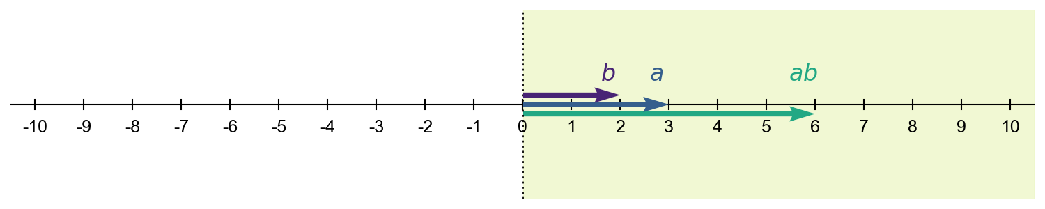
Positive definite matrices can be viewed as multivariate analogs to strictly positive real numbers, while positive semi-definite matrices can be viewed as multivariate analogs to nonnegative real numbers. Consider a scalar $a$. If $a < 0$, then the sign of $a b$ will depend on the sign of $b$. However, if $a > 0$, then $a b$ will have the same sign as $b$. We can think about $a$ and $b$ as $1$-vectors and about the product $ab$ as a dot product,

$\mathbf{a}^{\top} \mathbf{b} = \begin{bmatrix} a \end{bmatrix}^{\top} \begin{bmatrix} b \end{bmatrix} = ab. \tag{3}$

When $\mathbf{a}$ is positive, then $\mathbf{a}^{\top} \mathbf{b}$ will be on the same side of the origin $0$ as $\mathbf{b}$. So $\mathbf{a}$ does not “flip” $\mathbf{b}$ about the origin. Rather, it stretches $\mathbf{b}$ in the same direction (Figure $1$).

Figure 1. When $a > 0$, the product $ab$ can be interpreted as $b$ being stretched by $a$ in the same direction that $b$ already points, where $a$, $b$, and $ab$ are viewed as vectors with tails at the origin $0$. On the $y$-axis, vectors are offset from $0$ for visualization purposes.

Analogously, a positive definite matrix behaves like a positive number in the sense that it never flips a vector about the origin $\mathbf{0}$. The simplest example of a positive definite matrix is a diagonal matrix that scales a vector in the direction that it already points, and the simplest example of a matrix that is not positive definite is one which simply reverses the vector (Figure $2$).

Figure 2. (Left) A diagonal matrix $\mathbf{A}$ with positive diagonal values does not flip $\mathbf{x}$ about the origin and is thus positive definite. (Right) A diagonal matrix $\mathbf{A}$ with negative values flips $\mathbf{x}$ about the origin and is thus not positive definite.

However, it is less clear how to think about scenarios in which a matrix $\mathbf{A}$ projects a vector in a way that does not simply scale the vector by some constant. For example, does the matrix in the left subplot of Figure $3$ flip the vector $\mathbf{x}$ about the origin or not? What about the matrix in the middle subplot? How can we make these intuitions precise? The answer is in the dot product. The dot product between two $N$-vectors, defined as

$\mathbf{x}^{\top} \mathbf{y} = \sum_{n=1}^N x_n y_n, \tag{4}$

can be viewed as vector-matrix multiplication, which in turn can be viewed as a linear projection: an $N$-vector $\mathbf{y}$ is projected onto a real number line defined by the columns of a $1 \times N$ matrix $\mathbf{x}$. See my posts on matrices and the dot product if this claim does not make sense. Another definition of the dot product is that it is the product of the Euclidean magnitudes of the two vectors times the cosine of the angle between them:

$\mathbf{x}^{\top} \mathbf{y} = \lVert \mathbf{x} \rVert \lVert \mathbf{y} \rVert \cos \theta. \tag{5}$

What these definitions imply is that two nonzero vectors $\mathbf{x}$ and $\mathbf{y}$ are orthogonal to each other if their dot product is zero,

$\mathbf{x}^{\top} \mathbf{y} = 0. \tag{6}$

Why? First, if their dot product is zero and if neither vector is the zero vector, then the cosine angle between the two vectors must be $90^{\circ}$ (Figure $3$, middle).

Figure 3. A vector $\mathbf{x}$ is mapped by a matrix $\mathbf{A}$ to a new vector $\mathbf{Ax}$. (Left) The angle between $\mathbf{x}$ and $\mathbf{Ax}$ is acute. (Middle) The angle between $\mathbf{x}$ and $\mathbf{Ax}$ is right. The angle between $\mathbf{x}$ and $\mathbf{Ax}$ is obtuse.

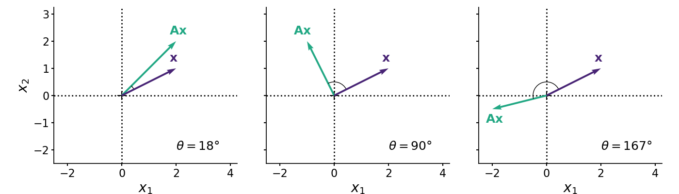
If the dot product between two nonzero vectors is positive,

$\mathbf{x}^{\top} \mathbf{y} > 0, \tag{7}$

then both vectors point in a “similar direction” in the sense that the cosine angle between them is less than $90^{\circ}$; the angle is acute (Figure $3$, left). And if the dot product is negative,

$\mathbf{x}^{\top} \mathbf{y} < 0, \tag{8}$

then both vectors point in a “dissimilar direction” in the sense that the cosine angle between them is greater than $90^{\circ}$; the angle is obtuse (Figure $3$, right).

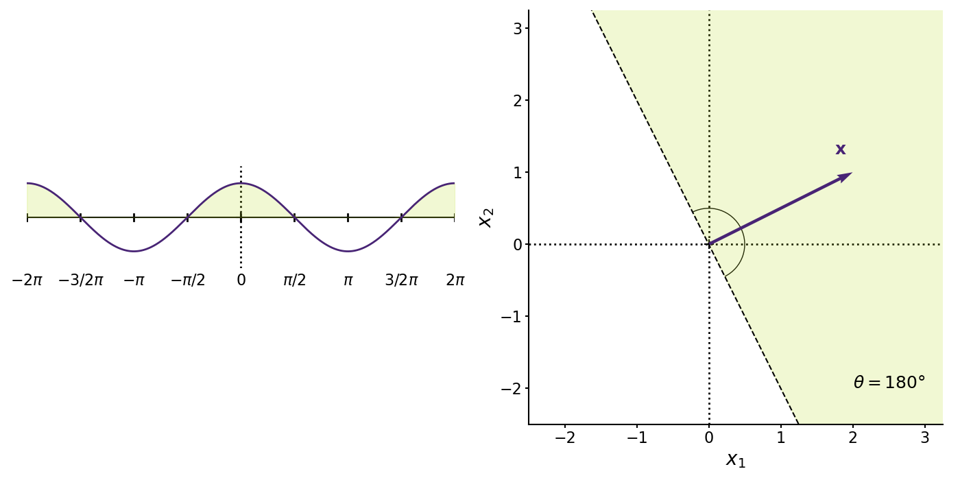
You can probably already see where we are going with this. One geometric interpretation of positive definiteness is that $\mathbf{A}$ does not “flip” $\mathbf{x}$ about the origin in the sense that the cosine angle between $\mathbf{x}$ and $\mathbf{A}\mathbf{x}$ is between $-90^{\circ}$ and $90^{\circ}$. In other words, $\mathbf{x}$ and $\mathbf{Ax}$ are in the same half of an $N$-dimensional hypersphere (Figure $4$).

Figure 4. (Left) The cosine function is positive between $-\pi/2$ and $\pi/2$ or between $-90^{\circ}$ and $90^{\circ}$. (Right) A positive semi-definite matrix $\mathbf{A}$ maps a vector $\mathbf{x}$ to a new location $\mathbf{Ax}$ such that the cosine angle between $\mathbf{x}$ and $\mathbf{Ax}$ is between $-90^{\circ}$ and $90^{\circ}$.

In my mind, Figure $4$ captures the geometric interpretation of Equation $1$. It’s a bit easier to see this when we make the location of the dot product operator more explicit, i.e.

$\mathbf{x} \cdot \mathbf{A}\mathbf{x} \gt 0. \tag{9}$

(Here, $\mathbf{a} \cdot \mathbf{b}$ is another common notation for the dot product.) This is similar to defining a real number as a number $a$ such that

$b(ab) > 0, \tag{10}$

for any number $b \neq 0$. To summarize everything so far, an $N \times N$ matrix is positive definite if it maps any vector into the same half of an $N$-dimensional hypersphere. Geometrically, this is analogous to a positive number (Figure $1$).

Examples

Now that we have a definition of and some geometric intuition for positive semi-definite matrices, let’s look at some examples. First, consider the matrix

$\mathbf{A} = \begin{bmatrix} 1 & 0 \\ 0 & 3 \end{bmatrix}. \tag{11}$

This is positive semi-definite since

$\begin{bmatrix} x_1 & x_2 \end{bmatrix} \begin{bmatrix} 1 & 0 \\ 0 & 3 \end{bmatrix} \begin{bmatrix} x_1 \\ x_2 \end{bmatrix} = x_1^2 + 3 x_2^2 \geq 0. \tag{12}$

We can see that it would be straightforward to prove that any diagonal matrix with positive elements is positive semi-definite. Since the diagonal elements in a diagonal matrix are the matrix’s eigenvalues, we might wonder if positive semi-definite matrices have nonnegative eigenvalues. Indeed, they do, which we’ll see in the next section.

Next, consider a singular matrix,

$\mathbf{A} = \begin{bmatrix} 1 & 1 \\ 1 & 1 \end{bmatrix}. \tag{13}$

This is positive semi-definite since

$\begin{bmatrix} x_1 & x_2 \end{bmatrix} \begin{bmatrix} 1 & 1 \\ 1 & 1 \end{bmatrix} \begin{bmatrix} x_1 \\ x_2 \end{bmatrix} = (x_1^2 + x_2)^2 \geq 0. \tag{14}$

Thus, a matrix does not need to be invertible to be positive semi-definite. However, we will see in the next section that a positive definite matrix must be invertible. As you might have guessed, this is because positive definite matrices must have strictly positive eigenvalues.

Now let’s look at an example of an indefinite matrix:

$\mathbf{A} = \begin{bmatrix} 1 & -2 \\ 2 & -1 \end{bmatrix}. \tag{15}$

This is indefinite since

$\begin{bmatrix} x_1 & x_2 \end{bmatrix} \begin{bmatrix} 1 & -2 \\ 2 & -1 \end{bmatrix} \begin{bmatrix} x_1 \\ x_2 \end{bmatrix} = x_1^2 - x_2^2 \ngeq 0. \tag{16}$

However, a matrix need not have negative entries to be indefinite. Consider this matrix with only positive values:

$\mathbf{A} = \begin{bmatrix} 3 & 5 \\ 5 & 4 \end{bmatrix}. \tag{17}$

Then

$\begin{bmatrix} x_1 & x_2 \end{bmatrix} \begin{bmatrix} 3 & 5 \\ 5 & 4 \end{bmatrix} \begin{bmatrix} x_1 \\ x_2 \end{bmatrix} = 3 x_1^2 + 10 x_1 x_2 + 4 x_2^2. \tag{18}$

Is this quadratic equation always positive? It’s hard to say because it’s not clear if the positive terms will grow faster than the potentially negative term, $10 x_1 x_2$. (In fact, this matrix is not positive semi-definite because for large enough values of $\mathbf{x}$, the quadratic $\mathbf{x}^{\top} \mathbf{A} \mathbf{x} \lt 0$.)

To me, these examples make clear that we need to understand some general mathematical properties that make identifying positive definiteness and positive semi-definiteness easier. Let’s do that now.

Properties

Positive semi-definite matrices have some convenient and important properties that make identifying and working with them relatively easy. I’ll only mention a few that come up often (for me). See (Bhatia, 2009) for a detailed discussion and rigorous proofs.

Eigenvalues. First, a positive definite matrix has strictly positive eigenvalues. Let $\mathbf{A}$ be an $N \times N$ matrix. Recall that the definition of the $n$-th eigenvector $\mathbf{v}_n$ with eigenvalue $\lambda_n$ is

$\mathbf{A} \mathbf{v}_n = \lambda_n \mathbf{v}_n. \tag{19}$

We can take the dot product between $\mathbf{v}_n$ and both sides of Equation $19$ to get

$\mathbf{v}_n^{\top} \mathbf{A} \mathbf{v}_n = \lambda_n \mathbf{v}_n^{\top} \mathbf{v}_n. \tag{20}$

If $\mathbf{A}$ is positive definite, then clearly $\lambda_n \gt 0$. Note that $\lambda_n \neq 0$, since this would imply that $\mathbf{v}_n^{\top} \mathbf{A} \mathbf{v}_n = 0$, which breaks our assumption about $\mathbf{A}$. In words, an eigenvector $\mathbf{v}_n$ of a matrix $\mathbf{A}$ is simply scaled by $\lambda_n$ when transformed by $\mathbf{A}$ (Figure $5$). Thus, $\lambda_n$ cannot be negative or else $\mathbf{A}\mathbf{v}_n$ could represent flipping $\mathbf{v}_n$ about the origin. Note that if $\mathbf{A}$ is positive semi-definite rather than positive definite, then the eigenvalues are nonnegative rather than strictly positive.

Figure 5. A matrix $\mathbf{A}$ with eigenvector $\mathbf{v}_n$ and eigenvalue $\lambda_n$. By definition, an eigenvector is a vector such that $\mathbf{Av}_n$ points in the same direction as $\mathbf{v}_n$ but with a magnitude defined by the eigenvalue $\lambda_n$.

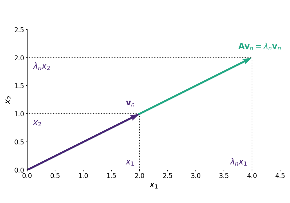
This is geometrically intuitive to me. We can think of the eigenvectors as defining how a matrix maps any vector transformed by the matrix, and the eigenvalues define the sign of each eigenvector. So if a matrix is to behave like a multivariate positive number, then the eigenvalues should be nonnegative so that the “action” of the matrix keeps the vector on the same side of the origin (as defined by Equation $1$ and visualized in Figure $4$).

We now have a straightforward way to verify that the matrix in Equation $17$ is not positive semi-definite. It has a negative eigenvalue:

>>> A = np.array([[3, 5], [5, 4]])
>>> eigvals, eigvecs = np.linalg.eig(A)
>>> any(eigvals < 0)
True

We can also easily check that the matrix in Equation $13$ is positive semi-definite, since it has nonnegative eigenvalues, but that it is not positive definite, since one eigenvalue is zero.

Determinant. Another way to think about this is via the determinant. Recall that the determinant of a matrix is the product of its eigenvalues,

$\det(\mathbf{A}) = \prod_{n=1}^N \lambda_n. \tag{21}$

The geometric intuition for the determinant of an $N \times M$ matrix is that it is the signed scale factor representing how much a matrix transforms the volume an $N$-cube into an $M$-dimensional parallelepiped. So if all the eigenvalues of a positive semi-definite matrix are nonnegative, then the determinant of a positive semi-definite matrix is nonnegative. This is just another way of quantifying what we mean by whether or not a matrix “flips” a vector about the origin.

So here is a second check that the matrix in Equation $17$ is not positive semi-definite. It has a negative determinant:

>>> A = np.array([[3, 5], [5, 4]])
>>> np.linalg.det(A)  # 3*4 - 5*5 = -13
-13.0

Decomposition. Recall that every positive number $a$ has two square roots, $\sqrt{a}$ and $-\sqrt{a}$. The positive square root is the principal square root, which is typically what is meant when someone refers to “the square root of $a$”. Analogously, every symmetric matrix $\mathbf{A}$ is positive semi-definite if and only if it can be decomposed as a product

$\mathbf{A} = \mathbf{B}^{\top} \mathbf{B}. \tag{22}$

Thus, $\mathbf{B}$ is the multivariate analog to the principal square root $\sqrt{a}$.

Let’s see why this is true. In the “only if” direction, let $\mathbf{A} = \mathbf{B}^{\top} \mathbf{B}$. Then

$\begin{aligned} \mathbf{x}^{\top} \mathbf{A} \mathbf{x} &= \mathbf{x}^{\top} \mathbf{B}^{\top} \mathbf{B} \mathbf{x} \\ &= \lVert \mathbf{B} \mathbf{x} \rVert_2^2 \\ &\geq 0. \end{aligned} \tag{23}$

This is similar to an argument that if $a = \sqrt{a}\sqrt{a}$, then $a$ is positive (for real numbers).

In the “if” direction, let $\mathbf{A}$ be a symmetric, positive semi-definite matrix. Since it is symmetric, it has an eigendecomposition

$\mathbf{A} = \mathbf{Q}\boldsymbol{\Lambda}\mathbf{Q}^{\top}, \tag{24}$

where $\mathbf{Q}$ is a $N \times N$ matrix of eigenvectors. Since $\mathbf{A}$ is positive semi-definite, all the eigenvalues are nonnegative. Thus, we can use $\boldsymbol{\Lambda}^{1/2}$ to denote a diagonal matrix, where each element in $\boldsymbol{\Lambda}^{1/2}$ is the square root of the associated eigenvalue in $\boldsymbol{\Lambda}$. Then $\mathbf{A}$ can be written as

$\mathbf{A} = \mathbf{Q}\boldsymbol{\Lambda}^{1/2}\boldsymbol{\Lambda}^{1/2}\mathbf{Q}^{\top}, \tag{25}$

and clearly $\mathbf{B} = \boldsymbol{\Lambda}^{1/2} \mathbf{Q}^{\top}$. This is why a convenient and fast way to construct a positive semi-definite matrix in code is to simply compute $\mathbf{B}^{\top} \mathbf{B}$ for a full-rank matrix $\mathbf{B}$.

>>> B = np.random.randn(100, 10)  # Construct full-rank matrix B.
>>> A = B.T @ B                   # Construct positive semi-definite matrix A.
>>> L = np.linalg.cholesky(A)     # Verify A is positive semi-definite.

I’m glossing over some finer points about the rank of $\mathbf{B}$ and the Cholesky decomposition here, but hopefully the main idea is clear.

We can now see why covariance matrices are positive semi-definite. The sample covariance is obviously positive semi-definite using the property above. If $\mathbf{X}$ is a full-rank design matrix with $N$ samples and $P$ predictors, then the sample covariance matrix,

$\hat{\boldsymbol{\Sigma}} = \frac{1}{N} \mathbf{X}^{\top} \mathbf{X}, \tag{26}$

is positive semi-definite matrix. We can also prove this is true for the population covariance. Let $\mathbf{x}$ be a random variable with mean $\boldsymbol{\mu}$ and population covariance

$\boldsymbol{\Sigma} = \mathbb{E}\left[(\mathbf{x} - \boldsymbol{\mu})(\mathbf{x} - \boldsymbol{\mu})^{\top}\right]. \tag{27}$

For any non-random vector, $\mathbf{w}$, we have

$\begin{aligned} \mathbf{w}^{\top} \boldsymbol{\Sigma} \mathbf{w} &= \mathbf{w}^{\top} \mathbb{E}\left[(\mathbf{x} - \boldsymbol{\mu})(\mathbf{x} - \boldsymbol{\mu})^{\top}\right] \mathbf{w} \\ &= \mathbb{E}\left[\mathbf{w}^{\top} (\mathbf{x} - \boldsymbol{\mu})(\mathbf{x} - \boldsymbol{\mu})^{\top} \mathbf{w} \right] \\ &= \mathbb{E}\left[ \left(\mathbf{w}^{\top} (\mathbf{x} - \boldsymbol{\mu})\right)^2 \right] \\ &\geq 0. \end{aligned} \tag{28}$

This works because the dot product is commutative. This is a result that is intuitive once we think of positive semi-definite matrices as nonnegative numbers. Since variance $\sigma^2$ is nonnegative, it makes sense that covariance $\boldsymbol{\Sigma}$ is positive semi-definite. And just as we can take the square root of $\sigma^2$, we can decompose the covariance $\boldsymbol{\Sigma}$.

Quadratic programming

There is a second geometric way to think about positive definite matrices: they are useful for optimization because an equation in quadratic form is convex when the matrix is symmetric and positive definite. Recall that a quadratic equation is any equation that can be written in the following form:

$f(x) = \frac{1}{2} ax^2 - bx + c. \tag{29}$

(As we will see in a moment, the coefficients $1/2$ and $-1$ just make the math a little cleaner for our purposes.) The generalization of a quadratic equation to multiple variables is any scalar-valued function in quadratic form:

$f(\mathbf{x}) = \frac{1}{2} \mathbf{x}^{\top} \mathbf{A} \mathbf{x} - \mathbf{b}^{\top} \mathbf{x} + c. \tag{30}$

What does this quadratic form have to do with definiteness? We will show that if $\mathbf{A}$ is a symmetric, positive-definite matrix, then $f(\mathbf{x})$ in Equation $30$ is minimized by the solution to $\mathbf{A} \mathbf{x} = \mathbf{b}$. This a very cool connection. It means that there are two ways of viewing $\mathbf{A}$. Let the notation $\mathbf{x}^{\star}$ denote the vector $\mathbf{x}$ that solves $\mathbf{A}\mathbf{x} = \mathbf{b}$. The claim is that

$\mathbf{x}^{\star} = \arg\!\min_{\mathbf{x}} \left\{ \frac{1}{2} \mathbf{x}^{\top} \mathbf{A} \mathbf{x} - \mathbf{b}^{\top} \mathbf{x} + c \right\}. \tag{31}$

This is fairly easy to prove, but let’s start with some geometric intuition.

First, observe that our claim is true in the univariate case. The first-order necessary condition for optimality is that the first derivative of $f$ is zero. We can find the critical points of $f$ by taking the derivative of $f$, setting it equal to zero, and solving for $x$:

$f^{\prime}(x) = 0 \implies x = \frac{b}{a}. \tag{32}$

So $x^{\star} = b/a$ satisfies the first-order condition for optimality. But is it a minimum? Let’s assume that $a > 0$, the univariate analog to positive definiteness. Then the second derivative $f^{\prime\prime}(x) = a$ is always positive:

$a \gt 0 \implies f^{\prime\prime}(x) \gt 0. \tag{33}$

Thus, $x^{\star}$ is a local minimum by the second derivative test. But notice we can make a stronger claim: $f$ is a convex function, since $f^{\prime\prime}(x) \gt 0$ for all $x$. So $x^{\star}$ is a global minimum (Figure $6$).

Figure 6. The quadratic function $f(x) = (1/2) a x^2 - bx + c$ for values $a = 6$, $b = 4$, and $c = -2$. The value $x = b/a = 2/3$ minimizes $f(x)$.

Now let’s look at the multivariate case. Perhaps you have already guessed what I will write next: just as $a$ must be positive for $f(x)$ to be the global minimum at $x = b/a$, the matrix $\mathbf{A}$ must be symmetric and positive definite for $f(\mathbf{x})$ to attain the global minimum at $\mathbf{x}^{\star}$. Let’s see that. Let $\mathbf{A}$ be a symmetric and positive matrix. Since it is symmetric, $\mathbf{A} = \mathbf{A}^{\top}$, and the derivative is

$\begin{aligned} f^{\prime}(\mathbf{x}) &= \frac{1}{2} \left( \mathbf{A} + \mathbf{A}^{\top} \right) \mathbf{x} - \mathbf{b} \\ &= \mathbf{A} \mathbf{x} - \mathbf{b}. \end{aligned} \tag{34}$

See Equation $81$ in (Petersen et al., 2008) for the derivative of $\mathbf{x}^{\top} \mathbf{A} \mathbf{x}$. So we can see that $\mathbf{x}^{\star}$ satisfies the first-order condition for optimality. And since the Hessian is positive definite, $f^{\prime\prime}(\mathbf{x}) = \mathbf{A}$,

$\mathbf{A} \succ 0 \implies f^{\prime\prime}(\mathbf{x}) \succ 0, \tag{35}$

then $\mathbf{x}^{\star}$ is a local minimum by the second partial derivative test. Finally, we can repeat our stronger claim: since the Hessian of $f$ is a positive definite for all $\mathbf{x}$, then $f$ is a convex function, and $\mathbf{x}^{\star}$ is the global minimum.

All that said, the above doesn’t provide much intuition as to why positive definiteness is the key property. Let’s try a different approach, which I found in (Shewchuk, 1994). Suppose that $\mathbf{A}$ is a symmetric matrix, and let $\mathbf{x} = \mathbf{x}^{\star}$. Let $\mathbf{e}$ be an “error term” in the sense that it is a random perturbation to $\mathbf{x}$. Then

$\begin{aligned} f(\mathbf{x} + \mathbf{e}) &= \frac{1}{2} (\mathbf{x} + \mathbf{e})^{\top} \mathbf{A} (\mathbf{x} + \mathbf{e}) - (\mathbf{x} + \mathbf{e})^{\top} \mathbf{b} + c \\ &= \frac{1}{2} \left[ \mathbf{x}^{\top} \mathbf{A} \mathbf{x} + \mathbf{e}^{\top} \mathbf{A} \mathbf{e} + 2 \mathbf{e}^{\top} \mathbf{A} \mathbf{x} \right] - \mathbf{x}^{\top} \mathbf{b} - \mathbf{e}^{\top} \mathbf{b} + c \\ &= \left( \frac{1}{2} \mathbf{x}^{\top} \mathbf{A} \mathbf{x} - \mathbf{x}^{\top} \mathbf{b} + c \right) + \frac{1}{2} \mathbf{e}^{\top} \mathbf{A} \mathbf{e} + \mathbf{e}^{\top} \mathbf{A} \mathbf{x} - \mathbf{e}^{\top}\mathbf{b} \\ &\stackrel{\star}{=} f(\mathbf{x}) + \frac{1}{2} \mathbf{e}^{\top} \mathbf{A} \mathbf{e} + \mathbf{e}^{\top} \mathbf{A} \mathbf{x} - \mathbf{e}^{\top} \mathbf{A} \mathbf{x} \\ &= f(\mathbf{x}) + \frac{1}{2} \mathbf{e}^{\top} \mathbf{A} \mathbf{e}. \end{aligned} \tag{36}$

Note that step $\star$, we again use the first-order condition for optimality when we replace $\mathbf{b}$ with $\mathbf{A} \mathbf{x}$. This derivation relies on the fact that when $\mathbf{A}$ is symmetric, $\mathbf{u}^{\top} \mathbf{A} \mathbf{v} = \mathbf{v}^{\top} \mathbf{A} \mathbf{u}$. So if $\mathbf{A}$ is a positive definite matrix, then $\mathbf{e}^{\top} \mathbf{A} \mathbf{e} \gt 0$. (Clearly, if $\mathbf{A}$ is positive semi-definite, then $\mathbf{e}^{\top} \mathbf{A} \mathbf{e} \geq 0$.) In my mind, this derivation helps explain why the critical point $\mathbf{x}^{\star}$ minimizes $f(\mathbf{x})$ when $\mathbf{A}$ is a positive definite matrix.

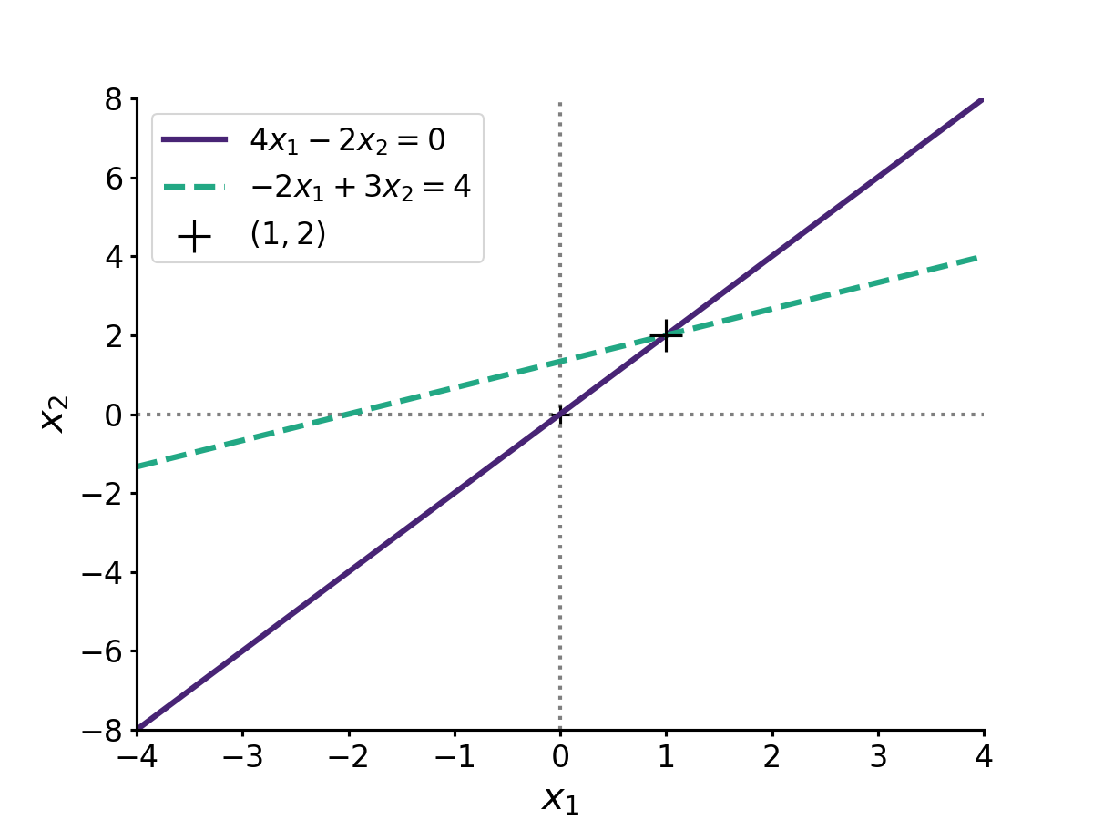
Now that we understand the math, let’s look at an example. Imagine, for example, that the values $\mathbf{A}$, $\mathbf{b}$ and $c$ are

$\mathbf{A} = \begin{bmatrix} 4 & -2 \\ -2 & 3 \end{bmatrix}, \qquad \mathbf{b} = \begin{bmatrix} 0 \\ 4 \end{bmatrix}, \qquad c = 5. \tag{37}$

We can easily confirm this is positive definite since its determinant is strictly positive. The solution of the linear system $\mathbf{A}\mathbf{x} = \mathbf{b}$ is

$\mathbf{x} = \begin{bmatrix} 1 \\ 2 \end{bmatrix}. \tag{38}$

Geometrically, the solution is just the point $\mathbf{x}$ where the two linear equations intersect, since this intersection is the point that satisfies both equations (Figure $7$).

Figure 7. The solution to the system of linear equations in Equation $37$ is the intersection of the two lines, $x_2 = 2 x_1$ and $x_2 = (1/3) x_1 + (4/3)$. The intersection is the point $[1, 2]$.

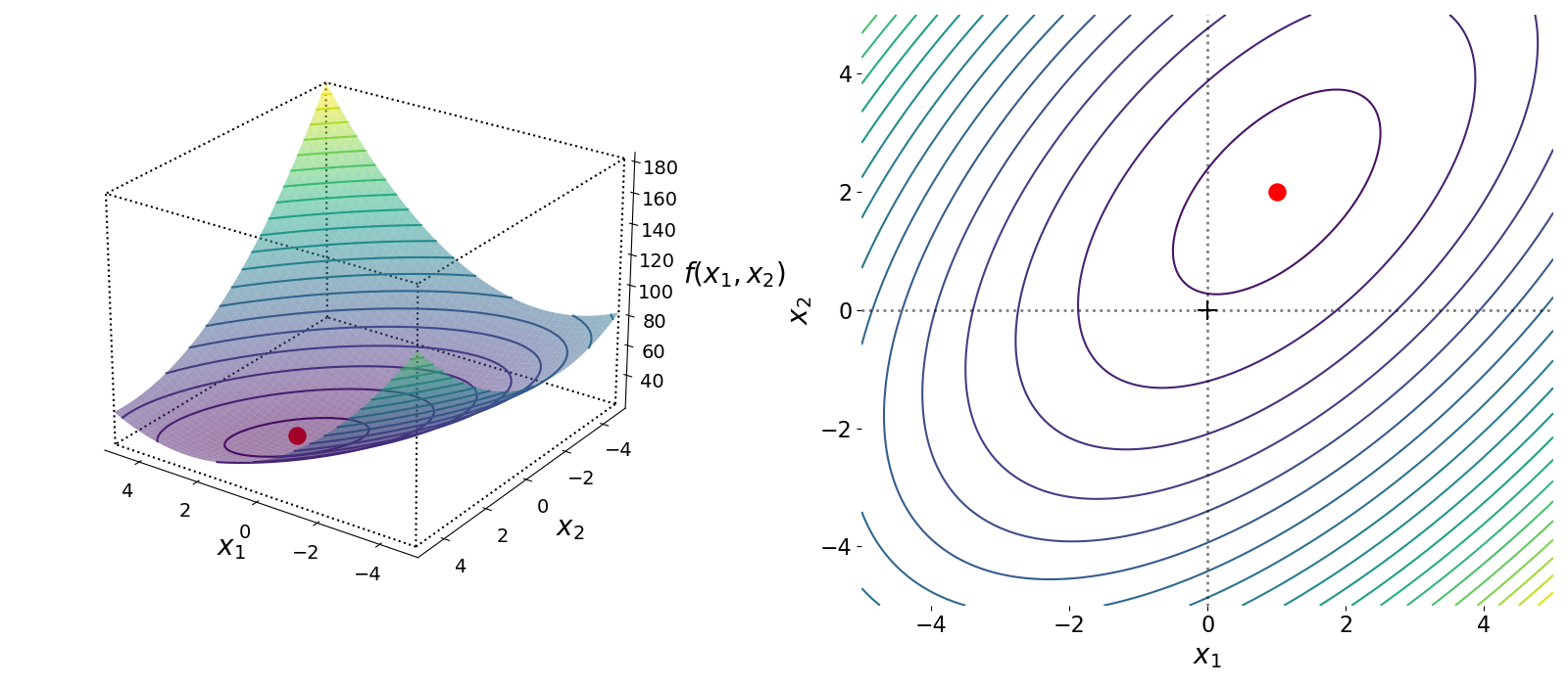
We proved above that this solution is the minimum point for the quadratic form in Equation $30$. We can visualize this function $f(\mathbf{x})$ in three-dimensions, $x_1$, $x_2$, and $f(x_1, x_2)$ where $\mathbf{x} = [ x_1, x_2 ]$. Geometrically, we can see that Equation $30$ is a convex function in three dimensions, and the point $\mathbf{x} = [ 1, 2 ]$ is the global minimum (Figure $8$).

Figure 8. Three-dimensional plot (left) and contour plot (right) of the function $f(\mathbf{x}) = (1/2) \mathbf{x}^{\top} \mathbf{Ax} - \mathbf{b}^{\top} \mathbf{x} + c$, with values defined by Equation $37$. The red dot indicates the solution to the equation $\mathbf{Ax} = \mathbf{b}$ (Equation $38$), which is also the global minimum.

Visualizing definiteness

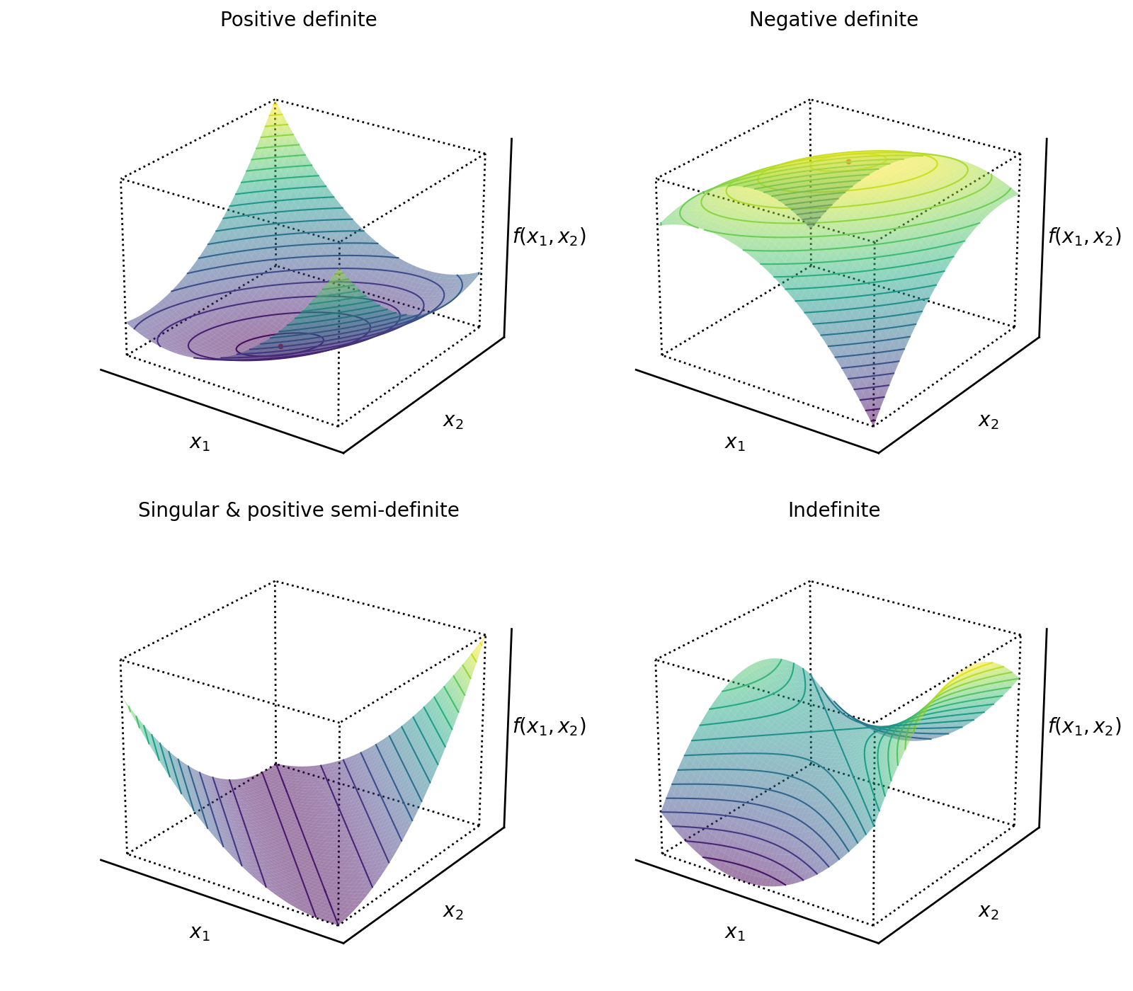
The previous example highlights a useful way to visualize the definiteness or indefiniteness of $2 \times 2$ matrices via the quadratic form in Equation $30$: we can plot the bivariate function

$f(x_1, x_2) = \frac{1}{2} \begin{bmatrix} x_1 & x_2 \end{bmatrix} \mathbf{A} \begin{bmatrix} x_1 \\ x_2 \end{bmatrix} - \mathbf{b}^{\top} \begin{bmatrix} x_1 \\ x_2 \end{bmatrix} + c \tag{39}$

in three dimensions to see how $f(x_1, x_2)$ changes for different types of matrices $\mathbf{A}$.

The quadratic form of a positive definite matrix is a convex function (Figure $10$, top left). The quadratic form of a negative matrix is a concave function (Figure $10$, top right). The quadratic form of a singular matrix is a function with a “trough”, since the linear system is overdetermined (has multiple solutions) (Figure $10$, bottom left). Singular matrices can be positive semi-definite provided the non-zero eigenvalues are positive. And the quadratic form of an indefinite matrix is a function with a saddle point (Figure $10$, bottom right).

Figure 9. Quadratic form with a positive definite matrix (top left), a negative definite matrix (top right), a singular yet positive semi-definite matrix (bottom left), and an indefinite matrix (bottom right).

Positive semi-definite cone

As a final note, the class of symmetric positive semi-definite matrices forms a “cone”, sometimes called the PSD cone. Mathematically, this is straightforward easy to see. Let $\mathbf{A}$ and $\mathbf{B}$ be two positive semi-definite matrices (not necessarily symmetric), and let $\alpha > 0$ and $\beta = 1 - \alpha$. Then

$\mathbf{x}^{\top} (\alpha \mathbf{A} + \beta \mathbf{B}) \mathbf{x} = \alpha \mathbf{x}^{\top} \mathbf{A} \mathbf{x} + \beta \mathbf{x}^{\top} \mathbf{B} \mathbf{x} \geq 0. \tag{40}$

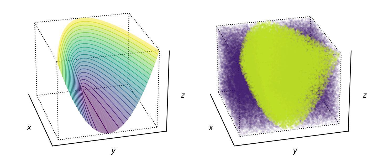
So the convex combination of two positive semi-definite matrices is itself a positive semi-definite matrix. This means that we can think of the space of all positive semi-definite matrices as a convex space. We can even visualize this in three dimensions for a two-dimensional matrix. Consider any arbitrary two dimensional symmetric matrix,

$\begin{bmatrix} x & z \\ z & y \end{bmatrix}. \tag{41}$

I have not proven it here, but one equivalent definition of a symmetric, positive semi-definite matrix is that all its leading principal minors are nonnegative. At a high-level, this captures the same idea as nonnegative eigenvalues or nonnegative determinant. This amounts to the constraint that

$x \geq 0, \qquad z^2 - xy \geq 0. \tag{42}$

So the surface of the positive semi-definite cone is

$xy = z^2, \tag{43}$

i.e. any positive semi-definite matrix will be “inside the cone” in the sense that if we plot its $(x, y, z)$ coordinates (as defined by Equation $41$) using Equation $42$, the location of the point will be inside the surface defined by Equation $43$ (Figure $10$).

Figure 10. (Left) The surface of the positive semi-definite cone for two-dimensional matrices. (Right) The positive semi-definite cone implied by sampling random positive semi-definite matrices and then plotting them in three-dimensions using the $(x, y, z)$ coordinates in Equation $41$.

Conclusion

An $N \times N$ positive definite matrix is analogous to a strictly positive number but in $N$-dimensional space, while a positive semi-definite matrix is analogous to a nonnegative number. This is because positive definite and positive semi-definite matrices transform vectors such that the output vector is in the same half of an $N$-dimensional hypersphere as the input vector. Positive semi-definite matrices have important properties, such nonnegative eigenvalues and a nonnegative determinant. Finally, positive definite matrices are important in optimization because a quadratic form with an $N \times N$ positive matrix is a convex function in $N+1$ dimensions

Acknowledgements

I thank for Melih Elibol for providing several detailed suggestions for clarifying this post.