Two Forms of the Dot Product

Two formulations

The dot product is an operation for multiplying two vectors to get a scalar value. Consider two vectors $\mathbf{a} = [ a_1, \dots, a_N ]$ and $\mathbf{b} = [ b_1, \dots, b_N ]$.¹ Their dot product is denoted $\mathbf{a} \cdot \mathbf{b}$, and it has two definitions, an algebraic definition and a geometric definition. The algebraic formulation is the sum of the elements after an element-wise multiplication of the two vectors:

$\mathbf{a} \cdot \mathbf{b} = a_1 b_1 + \dots + a_N b_N = \sum_{n=1}^{N} a_n b_n. \tag{1}$

The geometric formulation is the length of $\mathbf{a}$ multiplied by the length of $\mathbf{b}$ times the cosine of the angle between the two vectors:

$\mathbf{a} \cdot \mathbf{b} = \lVert \mathbf{a} \rVert \lVert \mathbf{b} \rVert \cos \theta, \tag{2}$

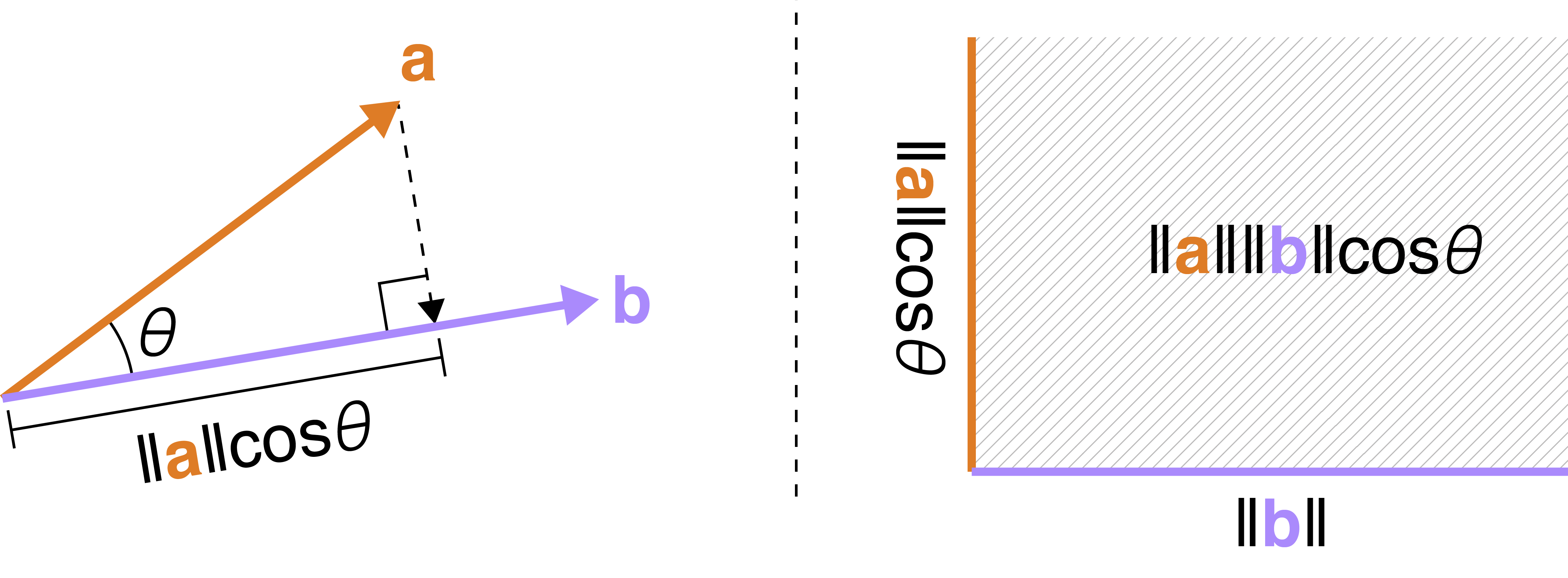
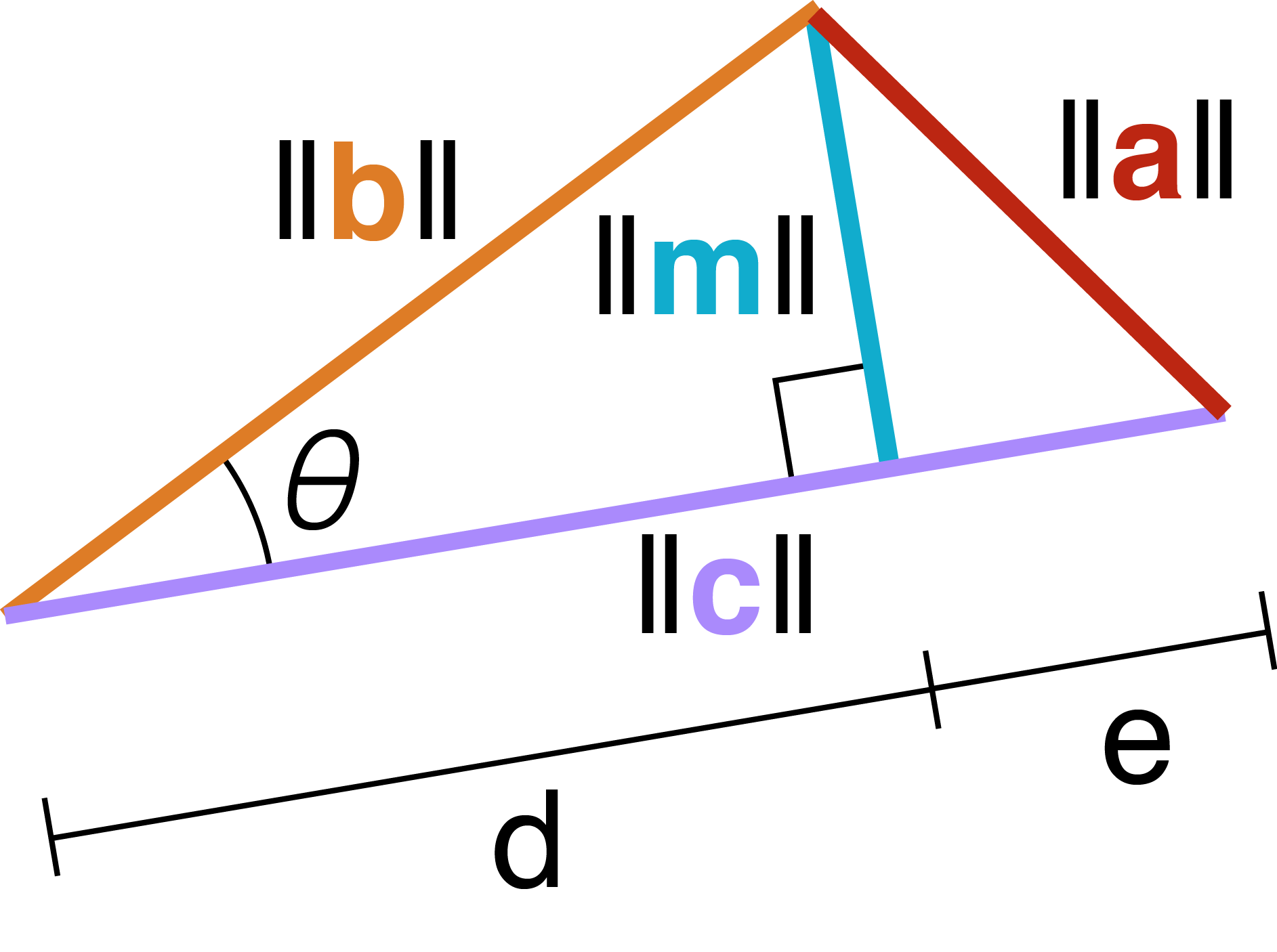
where $\lVert\mathbf{v}\rVert$ denotes the length (two-norm) of the vector $\mathbf{v}$. The geometric version can be easily visualized (Figure $1$) since

$\cos \theta = \frac{\text{adjacent}}{\text{hypotenuse $\lVert \mathbf{a} \rVert$}} \implies \lVert\mathbf{a}\rVert \cos \theta = \text{adjacent}. \tag{3}$

By the geometric definition, the dot product is the multiplication of the length of two vectors after one of the vectors ($\mathbf{a}$ in Figure $1$) has been projected onto the other one ($\mathbf{b}$ in Figure $1$).

Figure 1: The standard diagram of the dot product between vectors $\mathbf{a}$ and $\mathbf{b}$. The implication is that the dot product is the multiplication of the lengths of both vectors after one vector has been projected onto the other.

But how are these definitions related? (This StackOverflow has asked the same question with this amazing diagram.) How is the area in Figure $1$ related to a sum of element-wise products? The key is to realize that the summation in the algebraic definition is actually a linear projection. In this case, the dot product can be viewed as projecting a vector $\mathbf{a} \in \mathbb{R}^{N}$ by a matrix $\mathbf{b} \in \mathbb{R}^{1 \times N}$. As we explore this idea, I hope the geometric definition makes more sense as well.

Proof of equivalence

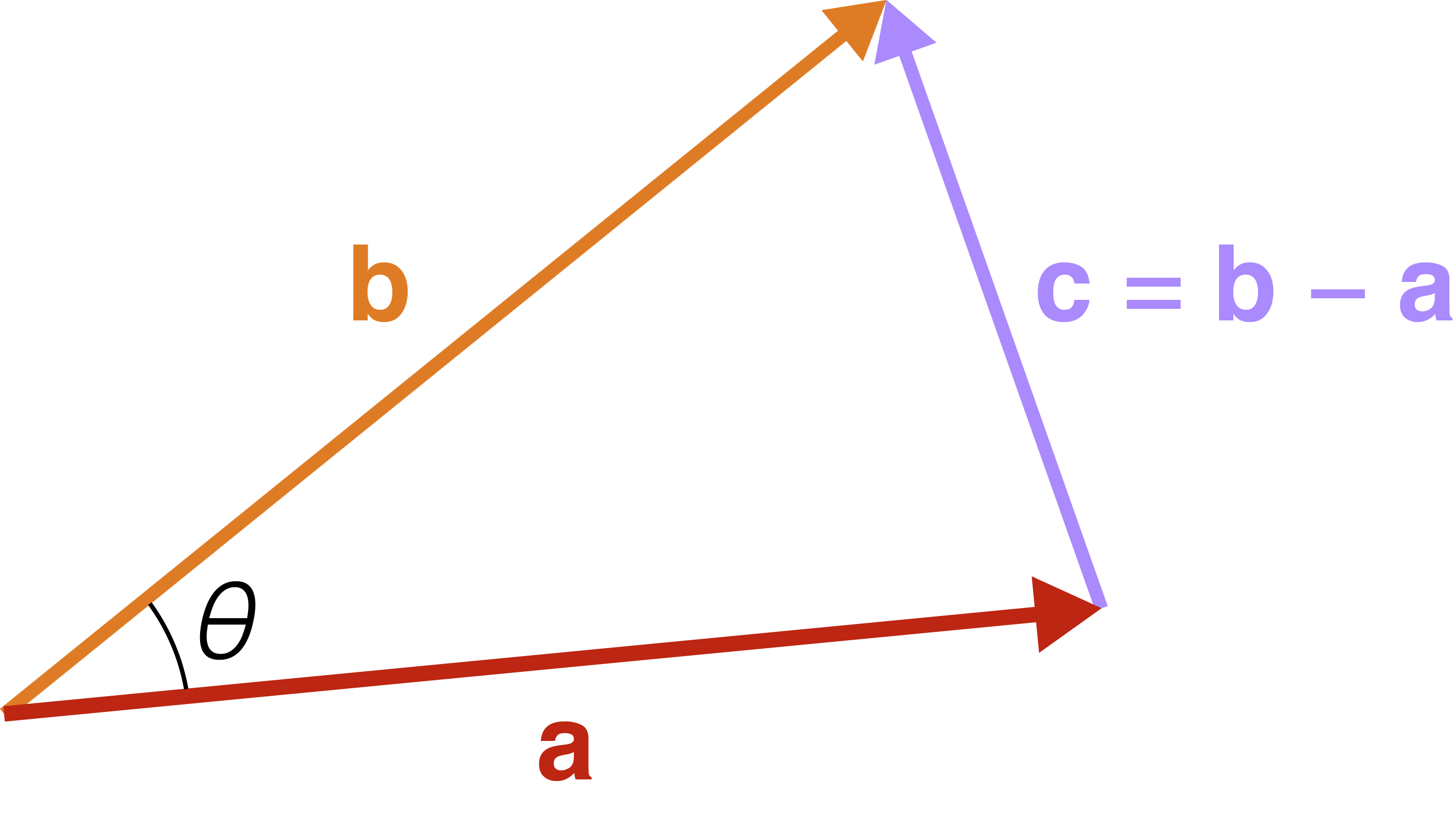
Before talking about the dot product as a linear projection, let’s quickly prove that the two definitions of the dot product are equivalent. This is based on Heidi Burgiel’s proof. Let’s assume the algebraic definition in Equation $1$. Then we want to prove Equation $2$. Define $\mathbf{c} := \mathbf{a} - \mathbf{b}$ (Figure $2$). Now notice that

$\begin{aligned} \lVert \mathbf{c} \rVert^2 &= \mathbf{c} \cdot \mathbf{c} \\ &= (\mathbf{a} - \mathbf{b}) \cdot (\mathbf{a} - \mathbf{b}) \\ &= \mathbf{a} \cdot \mathbf{a} - \mathbf{b} \cdot \mathbf{a} - \mathbf{a} \cdot \mathbf{b} + \mathbf{b} \cdot \mathbf{b} \\ &= \lVert \mathbf{a} \rVert^2 + \lVert \mathbf{b} \rVert^2 - 2 (\mathbf{a} \cdot \mathbf{b}). \end{aligned} \tag{4}$

Here, we used the commutative and distributive properties of the dot product (see A1 for proofs of these properties). This looks a lot like the law of cosines for the same triangle (see A2 for a proof of this law). We can readily see these two equations equal to each other and simplify:

$\begin{aligned} \lVert \mathbf{c} \rVert^2 &= \lVert\mathbf{c}\rVert^2 \\ \underbrace{\lVert\mathbf{a}\rVert^2 + \lVert\mathbf{b}\rVert^2 - 2 \mathbf{a} \cdot \mathbf{b}}_{\text{Equation $5$}} &= \underbrace{\lVert\mathbf{a}\rVert^2 + \lVert\mathbf{b}\rVert^2 - 2 \lVert\mathbf{a}\rVert \lVert\mathbf{b}\rVert \cos \theta}_{\text{Law of cosines}} \\ &\Downarrow \\ \mathbf{a} \cdot \mathbf{b} &= \lVert\mathbf{a}\rVert \lVert\mathbf{b}\rVert \cos \theta. \end{aligned} \tag{5}$

And we’re done. We have just proven that

$\sum_{n=1}^{N} a_n b_n = \lVert\mathbf{a}\rVert \lVert\mathbf{b}\rVert \cos \theta. \tag{6}$

However, this result is fairly counterintuitive to me, and my confusion as to how this could be true was the inspiration for this post. The geometric definition of the dot product is related to the law of cosines, which generalizes the Pythagorean theorem. But how is this definition related to the algebraic definition? Why are they both correct?

Figure 2: A geometric representation vector subtraction where $\mathbf{c} = \mathbf{a} - \mathbf{b}$.

Matrices as projections

The key to understanding the algebraic dot product is to understand how a matrix $\mathbf{M} \in \mathbb{R}^{P \times N}$ can be viewed as a linear transformation of $N$-dimensional vectors into a $P$-dimensional space. This is easiest to see with a $2 \times 2$ matrix, where we project a $2$-dimensional vector into another $2$-dimensional space. For example, consider the following vector $\mathbf{v}$ and linear transformation $\mathbf{M}$:

$\overbrace{\begin{bmatrix} \textcolor{#bc2612}{-7} & \textcolor{#11accd}{1} \\ \textcolor{#bc2612}{-5} & \textcolor{#11accd}{3} \end{bmatrix}}^{\mathbf{M}} \overbrace{\begin{bmatrix} 1 \\ 2 \end{bmatrix}}^{\mathbf{v}} = \overbrace{\begin{bmatrix} -5 \\ 1 \end{bmatrix}}^{\mathbf{Mv}}. \tag{7}$

Notice that the column vectors of $\mathbf{M}$ are actually the transformed standard basis vectors $\mathbf{e}_1$ and $\mathbf{e}_2$:

$\begin{bmatrix} \textcolor{#bc2612}{-7} & \textcolor{#11accd}{1} \\ \textcolor{#bc2612}{-5} & \textcolor{#11accd}{3} \end{bmatrix} \overbrace{\vphantom{\Bigg|} \begin{bmatrix} 1 \\ 0 \end{bmatrix} }^{\mathbf{e}_1} = \begin{bmatrix} \textcolor{#bc2612}{-7} \\ \textcolor{#bc2612}{-5} \end{bmatrix}, \qquad \begin{bmatrix} \textcolor{#bc2612}{-7} & \textcolor{#11accd}{1} \\ \textcolor{#bc2612}{-5} & \textcolor{#11accd}{3} \end{bmatrix} \overbrace{\vphantom{\Bigg|} \begin{bmatrix} 0 \\ 1 \end{bmatrix} }^{\mathbf{e}_2} = \begin{bmatrix} \textcolor{#11accd}{1} \\ \textcolor{#11accd}{3} \end{bmatrix}. \tag{8}$

And the projected vector $[ -5, 1 ]$ is just the original vector $[ 1, 2 ]$ using this new coordinate system specified by the transformed standard basis vectors, i.e.

$\begin{bmatrix} -5 \\ 1 \end{bmatrix} = 1 \overbrace{\begin{bmatrix} \textcolor{#bc2612}{-7} \\ \textcolor{#bc2612}{5} \end{bmatrix}}^{\mathbf{M} \mathbf{e}_1 } +2 \overbrace{\begin{bmatrix} \textcolor{#11accd}{1} \\ \textcolor{#11accd}{3} \end{bmatrix}}^{\mathbf{M} \mathbf{e}_2 }. \tag{9}$

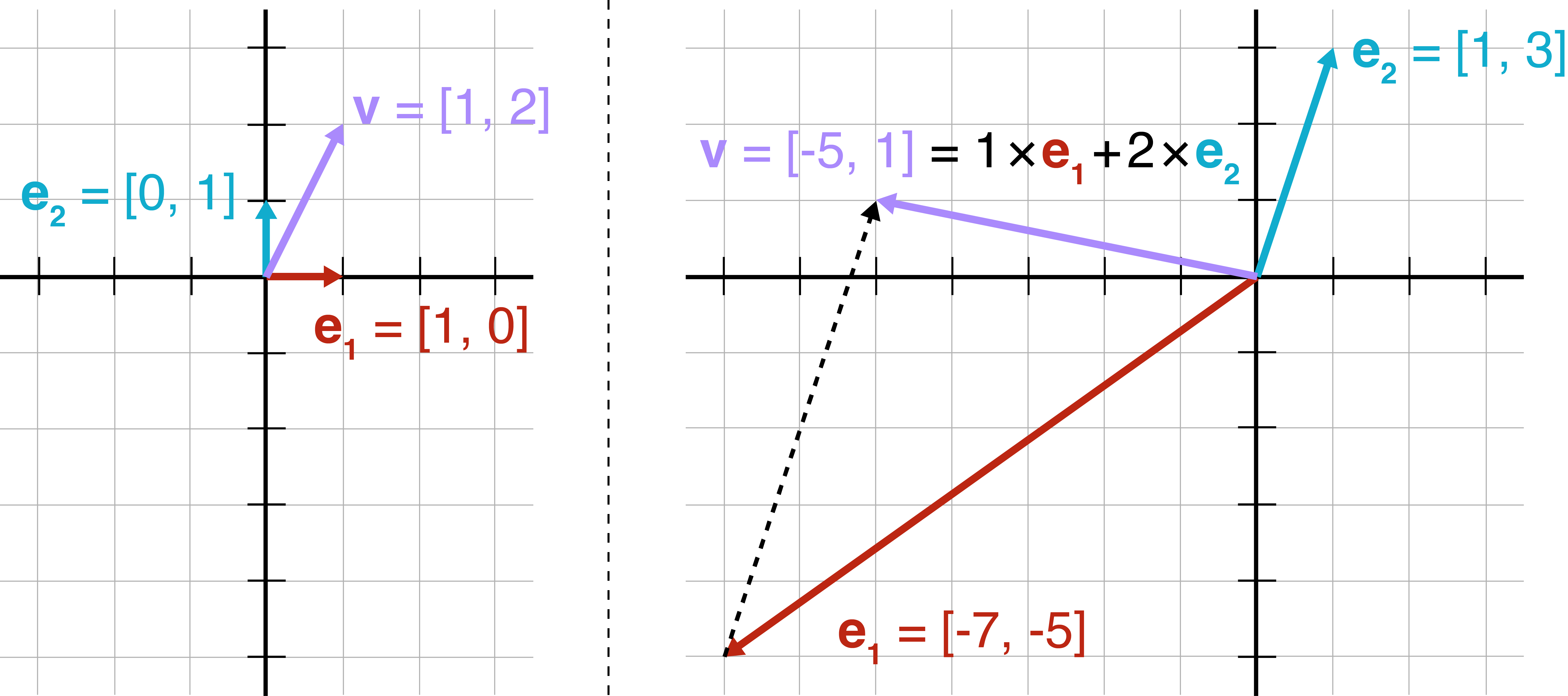
We can visualize this (Figure $3$) for some intuition. However, I highly recommend Grant Sanderson’s two beautiful explanations of linear projections and the dot product for interactive visualizations.

Figure 3: (Left) The vector $[ 1, 2 ]$ plotted in $2$-dimensional space with the standard basis vectors $\mathbf{e}_1 = [ 1, 0 ]$ and $\mathbf{e}_2 = [ 0, 1 ]$. (Right) The vector $[ 1, 2 ]$ transformed by the columns of $\mathbf{M}$, i.e. with the transformed standard basis vectors $\mathbf{Me}_1$ and $\mathbf{Me}_2$.

We can write this more generally. Consider the fact that we can represent any vector $\mathbf{v} = [v_1, \dots, v_N]$ as a linear combination of the standard basis vectors $\mathbf{e}_1, \dots, \mathbf{e}_N$:

$\mathbf{v} = v_1 \mathbf{e}_1 + \dots + v_N \mathbf{e}_N. \tag{10}$

This means we can apply our linear transformation $\mathbf{M}$ to get

$\mathbf{M}\mathbf{v} = v_1 (\mathbf{M} \mathbf{e}_1) + \dots + v_N (\mathbf{M} \mathbf{e}_N). \tag{11}$

So any $P$-vector $\mathbf{M} \mathbf{v}$ can be represented as a linear combination of the projected standard basis vectors $\mathbf{M}\mathbf{e}_1, \dots, \mathbf{M}\mathbf{e}_N$.

The dot product as a projection

We can think of the dot product as a matrix-vector multiplication where the left term is a $1 \times N$ matrix, i.e.,

$\mathbf{a} \cdot \mathbf{b} = \sum_{n=1}^N a_1 b_1 + \dots + a_N b_N = \begin{bmatrix} a_1 & \dots & a_N \end{bmatrix} \begin{bmatrix} b_1 \\ \vdots \\ b_N \end{bmatrix}. \tag{12}$

This is why the dot product is sometimes denoted as $\mathbf{a}^{\top} \mathbf{b}$ rather than as $\mathbf{a} \cdot \mathbf{b}$. So what does a $1 \times N$ matrix represent as a transformation? It is a transformation of $N$-vectors into a $1$-dimensional space, i.e. a line. So the dot product between vector $\mathbf{a}$ and $\mathbf{b}$ can be thought of as projecting $\mathbf{a} \in \mathbb{R}^N$ onto a number line defined by $\mathbf{b} \in \mathbb{R}^N$ (or vice versa). Our standard basis vectors are transformed such that they lie on a number line, and any vector projected into this new space must also lie on the number line. Each column in $\mathbf{b}$ is the $1$-dimensional analog to the standard basis vectors that we used in $\mathbb{R}^{N}$.

Let’s see a concrete example in $\mathbb{R}^2$. Let $\mathbf{a} = [3, 1]$ and $\mathbf{b} = [2, 4]$. Then the dot product between these two vectors can be written as a matrix-vector multiplication:

$\begin{bmatrix} 3 \\ 1 \end{bmatrix} \cdot \begin{bmatrix} 2 \\ 4 \end{bmatrix} = \begin{bmatrix} 3 & 1 \end{bmatrix} \begin{bmatrix} 2 \\ 4 \end{bmatrix} = \begin{bmatrix} 10 \end{bmatrix}. \tag{13}$

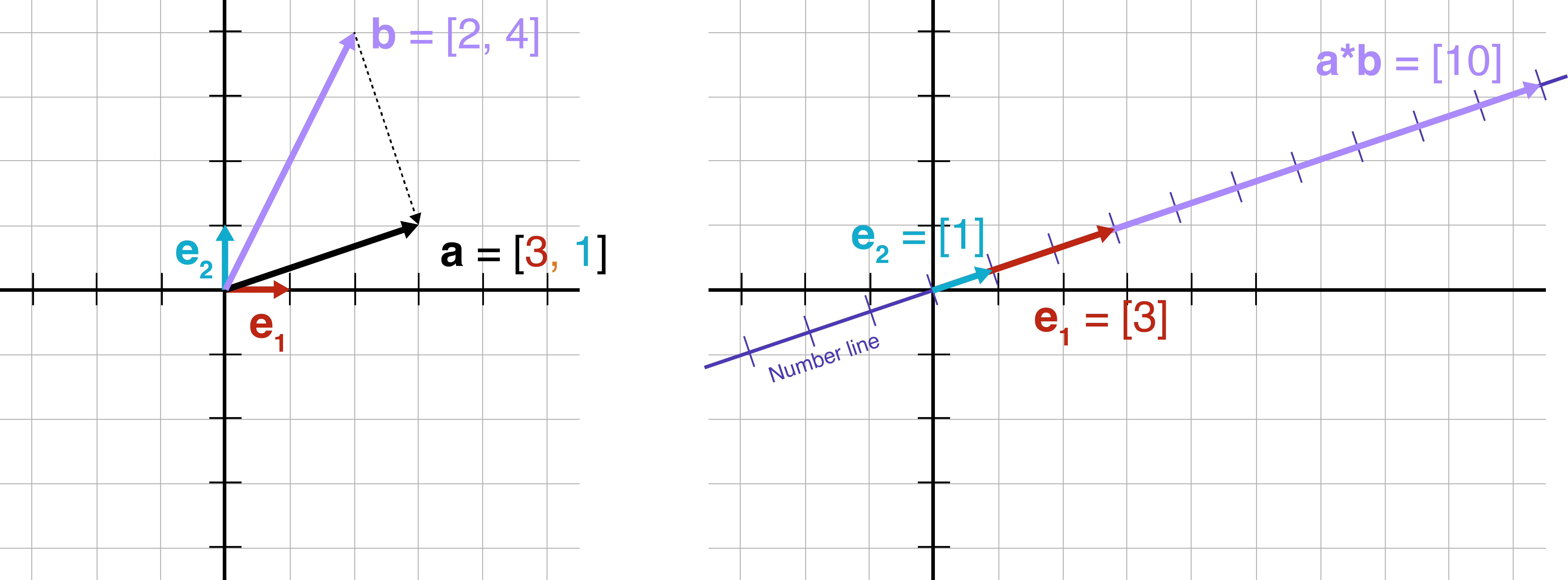
If we think about the dot product as a projection from $\mathbb{R}^2$ to $\mathbb{R}$, we can visualize the operation (Figure $4$). The $1$-vector $[10]$ is represented as a linear combination of the columns of $\mathbf{b} = [3, 1]$.

Figure 4: A vector $\mathbf{b} = [2, 4]$ projected onto a number line defined by a vector $\mathbf{a} = [3, 1]$.

As a sanity check, consider that points that are evenly spaced in $\mathbb{R}^2$ and then projected onto $\mathbf{a}$ will still be evenly spaced in $\mathbb{R}$. We can see this quantitatively. As we linearly scale either vector, we linearly scale the resultant value $\mathbf{a} \cdot \mathbf{b} = \alpha$:

$\begin{aligned} (k \mathbf{a}) \cdot \mathbf{b} &= \sum_{n=1}^N (k a_1) b_1 + \dots + (k a_N) b_N \\ &= k \left( \sum_{n=1}^N a_1 b_1 + \dots + a_N b_N \right) \\ &= k\alpha \end{aligned} \tag{14}$

While this is not a complete proof, this is the hallmark of a linear relationship.

Conclusion

How are the two definitions of the dot product related? The intuition is that both can be viewed as geometric operations. There are a lot of other good explanations of this idea online, but for me, the one that really made the idea click is realizing that the sum represents a linear projection.

Acknowledgments

I thank Stephen Talabac for pointing out some typos.

Appendix

A1. Proofs of commutative and distributive properties

The dot product is commutative because scalar multiplication is commutative:

$\begin{aligned} \mathbf{a} \cdot \mathbf{b} &= a_1 b_1 + a_2 b_2 + \dots + a_n b_n \\ &= b_1 a_1 + b_2 a_2 + \dots + b_n a_n \\ &= \mathbf{b} \cdot \mathbf{a}. \end{aligned} \tag{A.1}$

And the dot product is distributive because scalar multiplication is distributive:

$\begin{aligned} \mathbf{a} \cdot (\mathbf{b} + \mathbf{c}) &= \mathbf{a} \cdot [ (b_1 + c_1), (b_2 + c_2), \dots, (b_n + c_n) ]^{\top} \\ &= a_1 (b_1 + c_2) + a_2 (b_2 + c_2) + \dots + a_n (b_n + c_n) \\ &= a_1 b_1 + a_1 c_2 + a_2 b_2 + a_2 c_2 + \dots + a_n b_n + a_n c_n \\ &= (a_1 b_1 + a_2 b_2 + \dots + a_n b_n) + (a_1 c_1 + a_2 c_2 + \dots + a_n c_n) \\ &= \mathbf{a} \cdot \mathbf{b} + \mathbf{a} \cdot \mathbf{c}. \end{aligned} \tag{A.2}$

A2. Proof of the law of cosines

This is based on Sal Khan’s proof. The law of cosines is:

$\lVert\mathbf{c}\rVert^2 = \lVert\mathbf{a}\rVert^2 + \lVert \mathbf{b} \rVert^2 - 2 \lVert \mathbf{a} \rVert \lVert \mathbf{b} \rVert \cos \theta. \tag{A.3}$

Consider the triangle in Figure $5$.

Figure 5: An arbitary triangle.

Let’s first write $e$ and $\lVert \mathbf{m} \rVert$ in terms of $\cos$ and $\sin$:

$d := \lVert \mathbf{b} \rVert \cos(\theta), \qquad \lVert \mathbf{m} \rVert := \lVert \mathbf{b} \rVert \sin(\theta), \qquad e := \lVert \mathbf{c} \rVert - \underbrace{\lVert \mathbf{b} \rVert \cos(\theta)}_{d}. \tag{A.4}$

Now let’s use the Pythagorean theorem to construct a relationship between the sides:

$\begin{aligned} \lVert \mathbf{a} \rVert^2 &= \lVert \mathbf{m} \rVert^2 + e^2 \\ &= (\lVert \mathbf{b} \rVert \sin(\theta))^2 + (\lVert \mathbf{c} \rVert - \lVert \mathbf{b} \rVert \cos(\theta))^2 \\ &= \lVert \mathbf{b} \rVert^2 \sin^2(\theta) + \lVert \mathbf{c} \rVert^2 - 2 \lVert \mathbf{c} \rVert\lVert \mathbf{b} \rVert \cos(\theta) + \lVert \mathbf{b} \rVert^2 \cos^2(\theta) \\ &= \lVert \mathbf{b} \rVert^2 (\sin^2(\theta) + \cos^2(\theta)) + \lVert \mathbf{c} \rVert^2 - 2 \lVert \mathbf{c} \rVert \lVert \mathbf{b} \rVert \cos(\theta) \\ &= \lVert \mathbf{b} \rVert^2 + \lVert \mathbf{c} \rVert^2 - 2 \lVert \mathbf{c} \rVert\lVert \mathbf{b} \rVert \cos(\theta). \end{aligned} \tag{A.5}$

Note that the identity $\sin^2(\theta) + \cos^2(\theta) = 1$ is just the Pythagorean theorem applied to a right triangle inscribed inside a unit circle. Therefore, we have proven the law of cosines for an arbitrary triangle.