Singular Value Decomposition as Simply as Possible

Beyond the definition

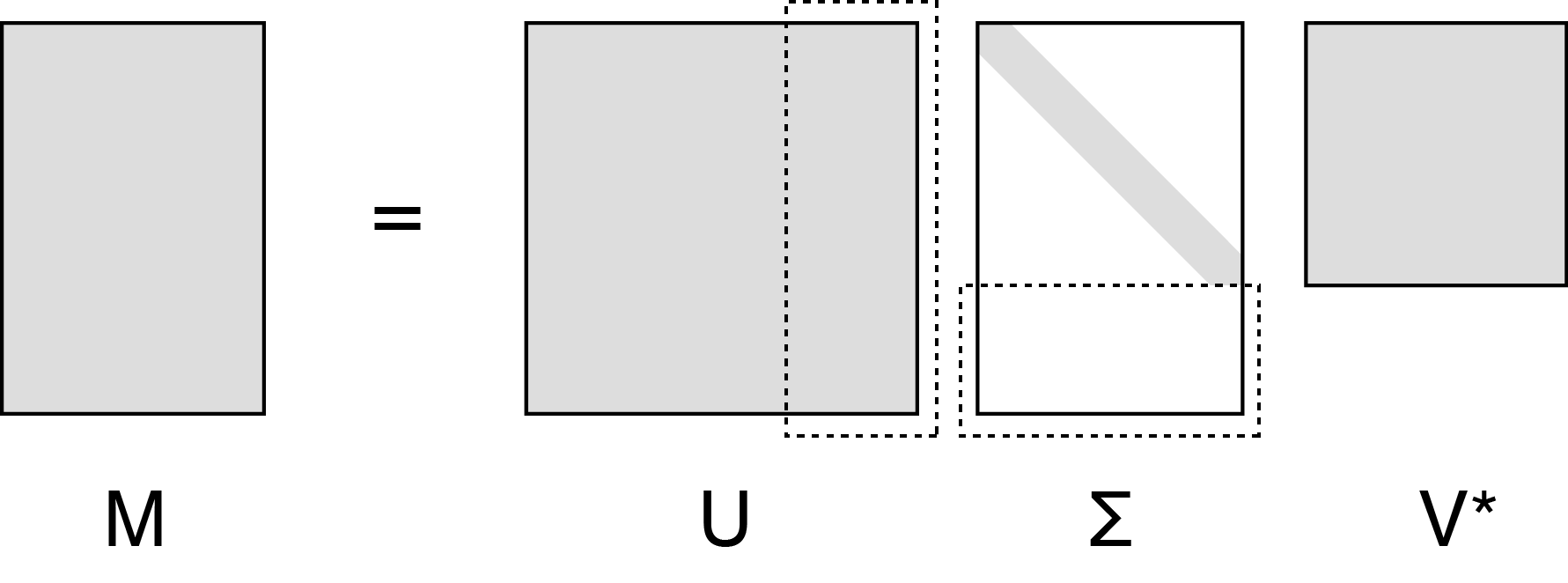
In my experience, the singular value decomposition (SVD) is typically presented in the following way: any matrix $\mathbf{M}\in {\mathbb{C}}^{m\times n}$ can be decomposed into three matrices,

$$\mathbf{M}=\mathbf{U}\mathbf{\Sigma }{\mathbf{V}}^{\ast }\text{\hspace{1em}(1)}$$

where $\mathbf{U}$ is an $m\times m$ unitary matrix, $\mathbf{\Sigma }$ is an $m\times n$ diagonal matrix, and $\mathbf{V}$ is an $n\times n$ unitary matrix. ${\mathbf{V}}^{\ast }$ is the conjugate transpose of $\mathbf{V}$. Depending on the source, the author may then take a few sentences to comment on how this equation can be viewed as decomposing the linear transformation $\mathbf{M}$ into two rotation and one dilation transformations or that a motivating geometric fact is that the image of a unit sphere under any $m\times n$ matrix is a hyperellipse. But how did we arrive at this equation and how do these geometrical intuitions relate to the equation above?

The goal of this post is simple: I want explain the SVD beyond this definition. Rather than present Equation $1$ in its final form, I want to build up to it from first principles. I will begin with an explanation of the SVD without jargon and then formalize the explanation to provide the definition in Equation $1$. Finally, I will discuss an application of the SVD that demonstrates its utility. In future posts, I hope to prove the existence and uniqueness of the SVD and explain randomized SVD in detail.

This post will rely heavily on a geometrical understanding of matrices. If you’re unfamiliar with that concept, please read my previous post on the subject.

SVD without jargon

Jargon is useful when talking within a community of experts, but I find that, at least for myself, it is easy to use jargon to mask when I do not understand something. If I were to present the SVD to a mathematician, the power of jargon is that I could convey the key ideas rapidly and precisely. The downside is that I could also simply use the words without fully understanding the underlying idea, while my expert listener filled in the gaps. As an exercise, I want to first present the SVD without jargon, as if explaining it to an interested 14-year-old—think eighth-grade level mathematical maturity. I will then formalize this intuitive explanation to work towards the standard formulation. So here we go.

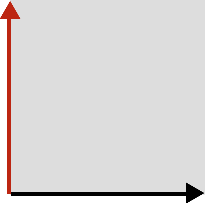
Imagine we have a square. The square, like your hand forming an “L”, has a particular orientation which we graphically represent with arrows (Figure $1$).

Figure 1: A square with orienting arrows.

We can manipulate this square in certain ways. For example, we can pull or push on an edge to stretch or compress the square (Figure 2A and 2B). We can rotate the square (Figure 2C) or flip it to change its orientation—imagine turning your hand over so that the “L” becomes an “⅃” (Figure 2D). We can even shear the square, which means to deform it by applying a force either up, down, left, or right at one of the square’s corners (Figure 2E).

Figure 2: Our original square under different types of transformations: (A) stretched, (B) compressed, (C) rotated, (D) reflected or flipped, and (E) sheared.

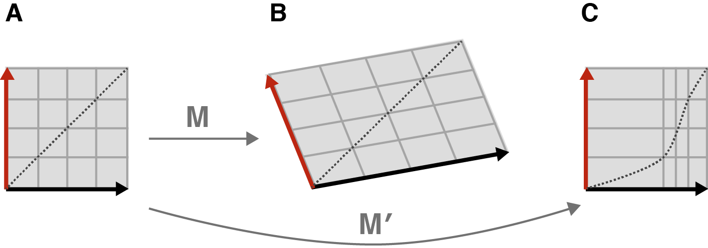
The only constraint is that our transformation must be linear. Intuitively, a linear transformation is one in which a straight line before the transformation results in a straight line after the transformation. To visualize what this means, imagine a grid of evenly spaced vertical and horizontal lines on our square. Now let’s draw a diagonal line on the square and perform some transformation. A linear transformation will be one such that after the transformation, this diagonal line is still straight (Figure 3B). To imagine the nonlinear transformation in Figure 3C, imagine bending a piece of engineering paper by pushing two sides together so that it bows in the middle.

Figure 3: (A) Our original square under a linear transformation $\mathbf{M}$ (B) and a nonlinear transformation ${\mathbf{M}}^{\prime }$ (C).

Now that we’ve defined our square and what we can do to it, we can state a cool mathematical fact. Consider any linear transformation $\mathbf{M}$, which we will apply to our square. If we are allowed to rotate our square before applying $\mathbf{M}$, then we can find a rotation such that, by first applying the rotation and then applying $\mathbf{M}$, we transform our square into a rectangle. In other words, if we rotate the square before applying $\mathbf{M}$, then $\mathbf{M}$ just stretches, compresses, or flips our square. We can avoid our square being sheared.

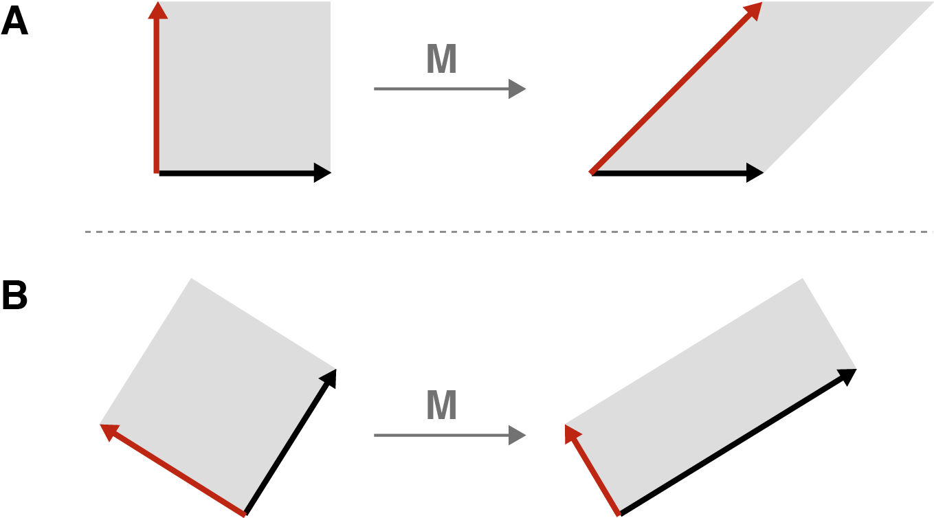
Let’s visualize this with an example. Imagine we sheared our square by pushing horizontally on its top left corner (Figure 4A). The result is a sheared square, kind of like an old barn tipping over. But if we rotated our square before pushing it sideways, the shear would result in only stretching and compressing the square, albeit in a new orientation (Figure 4B).

Figure 4: The geometric essence of the SVD: any linear transformation $\mathbf{M}$ of our square (A) can be thought of as simply stretching, compressing, or reflecting that square, provided we rotate the square before and after (B).

This is the geometric essence of the SVD. Any linear transformation can be thought of as simply stretching or compressing or flipping a square, provided we are allowed to rotate it first. The transformed square or rectangle may have a new orientation after the transformation.

Why is this a useful thing to do? The singular values referred to in the name “singular value decomposition” are simply the length and width of the transformed square, and those values can tell you a lot of things. For example, if one of the singular values is $0$, this means that our transformation flattens our square. And the larger of the two singular values tells you about the maximum “action” of the transformation.

If that second statement doesn’t make sense, consider visualizing our transformation without the second rotation, which does not effect the size of the rectangle in any way. (Imagine that rectangle in the bottom-right subplot of Figure 4 has the same orientation as the rotated square in the bottom-left subplot.) Also, instead of stretching (or flattening) a square into a rectangle, imagine stretching a circle into an ellipse (We’ll see why in a second.) (Figure 5).

Figure 5: (A) An oriented circle; if it helps, imagine that circle inscribed in our original square. (B) Our circle transformed into an ellipse. The length of the major and minor axes of the ellipse have values ${\sigma }_1$ and ${\sigma }_2$ respectively, called the singular values.

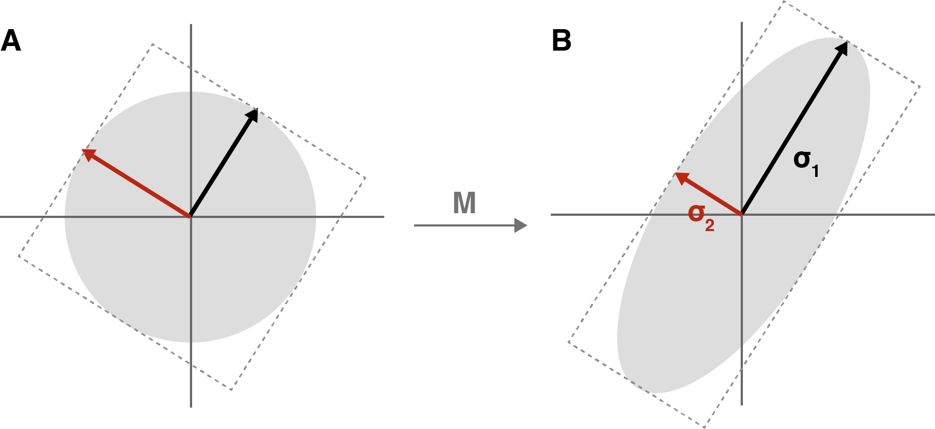
What does Figure 5 represent geometerically? The larger of the two singular values is the length of major axis of the ellipse. And since we transformed a perfect circle, every possible radii (the edge of the circle) has been stretched to the edge of the new ellipse. Which of these evenly-sized radii was stretched the most? The one pulled along the major axis. So the radius that was stretched the most was stretched an amount that is exactly equal to the largest singular value.

From intuition to definition

Now that we have a geometrical intuition for the SVD, let’s formalize these ideas. At this point, I am going to assume the reader is familiar with basic linear algebra. We want re-embrace jargon to speak precisely and efficiently.

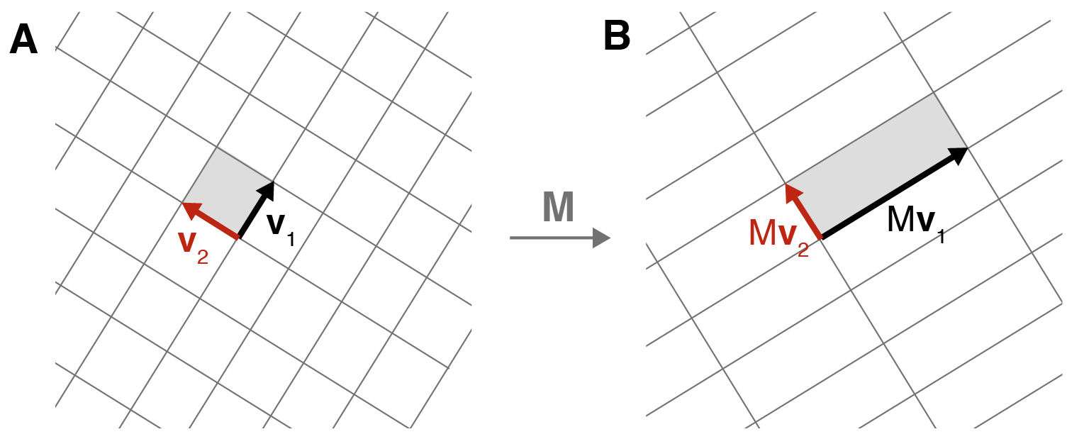
First, let’s name things. Recall that any pair of orthogonal unit vectors in two-dimensional space forms a basis for that space. In our case, let’s call the orthonormal vectors in the input space ${\text{v}}_1$ and ${\text{v}}_2$ (Figure 6A). After applying a matrix transformation $\mathbf{M}$ to these two vectors, we get $\mathbf{M}{\text{v}}_1$ and $\mathbf{M}{\text{v}}_2$ (Figure 6B). Furthermore, let’s decompose these two transformed vectors into unit vectors, ${\text{u}}_1$ and ${\text{u}}_2$, times their respective magnitudes, ${\sigma }_1$ and ${\sigma }_2$. In other words

$$\begin{array}{rl}\mathbf{M}{\text{v}}_1& ={\text{u}}_1{\sigma }_1,\\ \mathbf{M}{\text{v}}_2& ={\text{u}}_2{\sigma }_2.\end{array}\text{\hspace{1em}(2)}$$

So far, we have said nothing new. We are just naming things.

Figure 6: Formalizing the geometric essence of the SVD: if we properly rotate our domain defined by the basis vectors ${\text{v}}_1$ and ${\text{v}}_2$, then any linear transformation $\mathbf{M}$ is just a transformation by a diagonal matrix (dilating, reflecting) in a potentially rotated range defined by ${\text{u}}_1$ and ${\text{u}}_2$.

But now that we have things named, we can do a little algebraic manipulation. First, note that any vector $\text{x}$ can be described using the basis vectors ${\text{v}}_1$ and ${\text{v}}_2$ in the following way,

$$\text{x}=(\text{x}\cdot {\text{v}}_1){\text{v}}_1+(\text{x}\cdot {\text{v}}_2){\text{v}}_2\text{\hspace{1em}(3)}$$

where $\text{a}\cdot \text{b}$ denotes the dot product between vectors $\text{a}$ and $\text{b}$. If you’re unsure about the above formulation, consider a similar formulation with the standard basis vectors:

$$\begin{array}{rl}\text{x}& =(\text{x}\cdot {\text{e}}_1){\text{e}}_1+(\text{x}\cdot {\text{e}}_2){\text{e}}_2\\ & =x_1\left[\begin{array}{c}1\\ 0\end{array}\right]+x_2\left[\begin{array}{c}0\\ 1\end{array}\right].\end{array}\text{\hspace{1em}(4)}$$

where $x_i$ denotes the $i$-th component of $\text{x}$. In Equation $3$, we are projecting, via the dot product, $\text{x}$ onto ${\text{v}}_1$ and ${\text{v}}_2$, before decomposing the terms using the basis vectors ${\text{v}}_1$ and ${\text{v}}_2$.

Next, let’s left-multiply both sides of Equation $3$ by our matrix transformation $\mathbf{M}$. Since the dot product is a scalar, we can distribute and commute $\mathbf{M}$ as follows:

$$\mathbf{M}\text{x}=(\text{x}\cdot {\text{v}}_1)\mathbf{M}{\text{v}}_1+(\text{x}\cdot {\text{v}}_2)\mathbf{M}{\text{v}}_2.\text{\hspace{1em}(5)}$$

Next, we can rewrite $\mathbf{M}{\text{v}}_i$ as ${\text{u}}_i{\sigma }_i$:

$$\mathbf{M}\text{x}=(\text{x}\cdot {\text{v}}_1){\text{u}}_1{\sigma }_1+(\text{x}\cdot {\text{v}}_2){\text{u}}_2{\sigma }_2.\text{\hspace{1em}(6)}$$

We’re almost there. Now since the dot product is commutative, we can switch the ordering, e.g. $\text{x}\cdot {\text{v}}_1=\text{x}\cdot {\text{v}}_1={\text{v}}_1\cdot \text{x}$. And since each dot product term is a scalar, we move each one to the end of their respective expressions:

$$\mathbf{M}\text{x}={\text{u}}_1{\sigma }_1\left({\text{v}}_1\cdot \text{x}\right)+{\text{u}}_2{\sigma }_2\left({\text{v}}_2\cdot \text{x}\right).\text{\hspace{1em}(7)}$$

Now we can remove $\text{x}$ from both sides of the equation because, in general,

$$\mathbf{A}\mathbf{x}=\mathbf{B}\mathbf{x}⟹\mathbf{A}=\mathbf{B}.\text{\hspace{1em}(8)}$$

For details, see the discussion here. It might be easier to intuit if we rewrite the claim as

$$(\mathbf{A}-\mathbf{B})\mathbf{x}=0⟹\mathbf{A}-\mathbf{B}=0.\text{\hspace{1em}(9)}$$

Removing $\mathbf{x}$, we get:

$$\mathbf{M}={\text{u}}_1{\sigma }_1{\text{v}}_1^{\ast }+{\text{u}}_2{\sigma }_2{\text{v}}_2^{\ast }\text{\hspace{1em}(10)}$$

Given appropriately defined matrices, Equation $10$ becomes the SVD in its canonical form (Equation $1$) for $2\times 2$ matrices:

$$\mathbf{M}=\underset{\mathbf{M}}{\underbrace{\left[\begin{array}{cc}{\text{u}}_1& {\text{u}}_2\end{array}\right]}}\underset{\mathbf{\Sigma }}{\underbrace{\left[\begin{array}{cc}{\sigma }_1& 0\\ 0& {\sigma }_2\end{array}\right]}}\underset{{\mathbf{V}}^{\ast }}{\underbrace{\left[\begin{array}{c}{\text{v}}_1^{\ast }\\ {\text{v}}_2^{\ast }\end{array}\right]}}\text{\hspace{1em}(11)}$$

Furthermore, you should have an intuition for what this means. Any matrix transformation can be represented as a diagonal transformation (dilating, reflecting) defined by $\mathbf{\Sigma }$ provided the domain and range are properly rotated first.

The vectors ${\text{u}}_i$ are called the left singular vectors, while the vectors ${\text{v}}_i$ are called the right singular vectors. This orientating terminology is a bit confusing because “left” and “right” come from the equation above, while in our diagrams of rectangles and ellipses, the ${\text{v}}_i$ vectors are on the left.

The standard formulation

Now that we have a simple geometrical intuition for the SVD and have formalized it for all $2\times 2$ matrices, let’s re-formulate the problem in general and in the standard way. If jumping from $2$-dimensions to $n$-dimensions is challenging, recall the advice of Geoff Hinton:

To deal with hyper-planes in a 14-dimensional space, visualize a 3-D space and say “fourteen” to yourself very loudly. Everyone does it.

Consider that given our definitions of ${\text{v}}_i$, ${\text{u}}_i$, and ${\sigma }_i$, we can rewrite Equation $2$ for an arbitrary $m\times n$ matrix $\mathbf{M}$ as:

$$\left[\begin{array}{ccccc}& & & & \\ & & & & \\ & & \mathbf{M}& & \\ & & & & \\ & & & & \end{array}\right]\left[\begin{array}{ccc}& & \\ {\text{v}}_1& \dots & {\text{v}}_n\\ & & \end{array}\right]=\left[\begin{array}{ccc}& & \\ & & \\ {\text{u}}_1& \dots & {\text{u}}_m\\ & & \\ & & \end{array}\right]\left[\begin{array}{ccc}{\sigma }_1& & \\ & \ddots & \\ & & {\sigma }_n\\ & & \end{array}\right]\text{\hspace{1em}(12)}$$

which immediately gives us Equation $11$ again, but for $m\times n$ matrices:

$$\begin{array}{rl}\mathbf{M}\mathbf{V}& =\mathbf{U}\mathbf{\Sigma }\\ {\mathbf{M}\mathbf{V}\mathbf{V}}^{\ast }& =\mathbf{U}\mathbf{\Sigma }{\mathbf{V}}^{\ast }\\ \mathbf{M}& =\mathbf{U}\mathbf{\Sigma }{\mathbf{V}}^{\ast }\end{array}\text{\hspace{1em}(13)}$$

Here, $\mathbf{U}$ is unitary and $m\times m$; $\mathbf{V}$ is unitary and $n\times n$; and $\mathbf{\Sigma }$ is diagonal and $m\times n$. ${\mathbf{V}\mathbf{V}}^{\ast }=\mathbf{I}$ since $\mathbf{V}$ is orthonormal. This is schematically drawn in Figure 7.

Figure 7: The canonical diagram of the SVD decomposition of a matrix $\mathbf{M}$. The columns of $\mathbf{U}$ are the orthonormal left singular vectors; $\mathbf{\Sigma }$ is a diagonal matrix of singular values; and the rows of ${\mathbf{V}}^{\ast }$ are the orthonormal right singular vectors. The dashed areas are padding.

The diagonal elements of $\mathbf{\Sigma }$ are the singular values. Without loss of generality, we can assume the singular values are ordered—ordering them might require reordering the columns of $\mathbf{U}$ and $\mathbf{V}$. And the geometric interpretation of them holds in higher dimensions. For example, if we performed the SVD on an $m\times n$ matrix and noticed that the bottom $k$ singular values were smaller than some epsilon, you could visualize this matrix transformation as flattening a hyperellipse along those $k$ dimensions. Or if you have an exponential decay in the value of the singular values, it suggests that all the “action” of the matrix happens along only a few dimensions.

And that’s it! That’s the SVD. You can read about the distinction between the full and truncated SVD, about handling low-rank matrices, and so forth in better resources than this. My goal was to arrive at Equation $1$ through as simple reasoning as possible. At least in my opinion, going slowly through the geometrical intuition makes explanations of the SVD make more sense.

Re-visualizing the SVD

Now that we understand the SVD, we can convince ourselves that we have been visualizing it correctly. Consider Figure 8, which was generated using Matplotlib and NumPy’s implementation of the SVD, numpy.linalg.svd. We can see that these figures exactly match our intuition for what is happening for the SVD in $2$-dimensions.

Figure 8: Several examples of using NumPy's implementation of the SVD to visualize the algorithm. Each frame has two pairs of overlaid rectangles. For each pair, a square is transformed into a parallelogram by a linear transformation. In the left pair, the square is unrotated. In the right pair, the square is rotated by $\mathbf{V}$ before applying the transformation. Each dashed line is the top singular vector for the associated transformation.

Applications

The SVD is related to many other matrix properties. The number of nonzero singular values is equal to the rank of the matrix. This is why the spectral norm is a convex surrogate for low-rank approximations. The range of a matrix is the space spanned by the vectors $\{{\text{u}}_1,{\text{u}}_2,\dots ,{\text{u}}_r\}$ where $r$ is the number of nonzero singular values and all the singular values and vectors are ordered. A matrix is uninvertible if it has a singular value that is zero because the transformation is “collapsing” an $n$-cube along at least one dimension. And so on. Once the SVD is understood, I think it’s fairly straightforward to intuit why the aforementioned properties must hold. See Chapter 5 of (Trefethen & Bau III, 1997) for details.

One algorithm I find much easier to understand after understanding SVD is principal component analysis (PCA). Rather than assume you know how PCA works, let’s look at what PCA computes and then let’s reason about what PCA is doing with our knowledge of the SVD. Consider a real-valued data matrix $\mathbf{X}$ that is $n\times p$ where $n$ is the number of samples and $p$ is the number of features. Its SVD is

$$\mathbf{X}=\mathbf{U}\mathbf{\Sigma }{\mathbf{V}}^{\top }.\text{\hspace{1em}(12)}$$

Now consider the covariance matrix of $\mathbf{X}$, namely ${\mathbf{X}}^{\top }\mathbf{X}$, in the context of the SVD decomposition:

$$\begin{array}{rl}{\mathbf{X}}^{\top }\mathbf{X}& =(\mathbf{U}\mathbf{\Sigma }{V}^{\top }{)}^{\top }(\mathbf{U}\mathbf{\Sigma }{\mathbf{V}}^{\top })\\ & =\mathbf{V}{\mathbf{\Sigma }}^{\top }{\mathbf{U}}^{\top }\mathbf{U}\mathbf{\Sigma }{\mathbf{V}}^{\top }\\ & =\mathbf{V}{\mathbf{\Sigma }}^{\top }\mathbf{\Sigma }{\mathbf{V}}^{\top }\\ & =\mathbf{V}{\mathbf{\Sigma }}^2{\mathbf{V}}^{\top }\end{array}\text{\hspace{1em}(13)}$$

We already know that $\mathbf{V}$ and ${\mathbf{V}}^{\top }$ are just rotation matrices, while $\mathbf{U}$ disappears because ${\mathbf{U}}^{\top }\mathbf{U}=\mathbf{I}$. And even without knowing about eigenvectors or eigenvalues, we can see what PCA is doing by understanding SVD: it is diagonalizing the covariance matrix of $\mathbf{X}$. So PCA is finding the major axes along which our data varies.

If it’s not clear what SVD or eigendecomposition on data means, Jeremy Kun has a good blog post about that.

Conclusion

The singular value decomposition or SVD is a powerful tool in linear algebra. Understanding what the decomposition represents geometrically is useful for having an intuition for other matrix properties and also helps us better understand algorithms that build on the SVD.

Acknowledgments

Writing this post required that I synthesize from a number of excellent resources. Most notably, for the derivation in the section formalizing the SVD, I used this tutorial from the American Mathematical Society. I thank Mahmoud Abdelkhalek and Alfredo Canziani for bringing errata to my attention.