Canonical Correlation Analysis in Detail

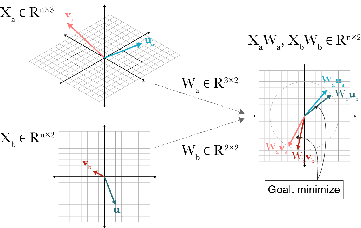
Canonical correlation analysis (CCA) is a multivariate statistical method for finding two linear projections, one for each set of observations in a paired dataset, such that the projected data points are maximally correlated. Provided the data are mean-centered, this procedure can be visualized fairly easily (Figure $1$). CCA finds linear projections such that paired data points are close to each other in a lower-dimensional space. And since mean-centered points are vectors with tails at $(0,0)$, CCA can be thought of as minimizing the cosine distance between paired points.

Figure 1: A visualization of canonical correlation analysis. Let $n=2$ be the number of observations. Two datasets ${\mathbf{X}}_a\in {\mathbb{R}}^{n\times 3}$ and ${\mathbf{X}}_b\in {\mathbb{R}}^{n\times 2}$ are transformed by projections $W_a\in {\mathbb{R}}^{3\times 2}$ and $W_b\in {\mathbb{R}}^{2\times 2}$ such that the paired embeddings, $({\text{v}}_a,{\text{v}}_b)$ and $({\text{u}}_a,{\text{u}}_b)$, are maximally correlated with unit length in the projected space.

The goal of this post is to go through the CCA procedure in painstaking detail, denoting the dimensionality of every vector and matrix, explaining the objective and constraints, walking through a derivation that proves how to solve the objective, and providing working code.

CCA objective

Consider two paired datasets, ${\mathbf{X}}_a\in {\mathbb{R}}^{n\times p}$ and ${\mathbf{X}}_b\in {\mathbb{R}}^{n\times q}$. By “paired”, I mean that the $i$-th sample consist of two row vectors, $({\text{x}}_a^i,{\text{x}}_b^i)$, with dimensionality $p$ and $q$ respectively. Thus, there are $n$ paired empirical multivariate observations. We assume the data are mean-centered. See the Appendix, Section 1 for a mathematical discussion of what this means.

Let ${\text{w}}_a\in {\mathbb{R}}^p$ and ${\text{w}}_b\in {\mathbb{R}}^q$ denote linear transformations of the data (note that these are vectors and not matrices, as in Figure $1$; this will be explained). A pair of canonical variables ${\text{z}}_a\in {\mathbb{R}}^n$ and ${\text{z}}_b\in {\mathbb{R}}^n$ are the images of ${\mathbf{X}}_a$ and ${\mathbf{X}}_b$ after projection, i.e.:

$${\text{z}}_a={\mathbf{X}}_a{\text{w}}_a{\text{z}}_b={\mathbf{X}}_b{\text{w}}_b$$

The goal of CCA is to learn linear transformations ${\text{w}}_a$ and ${\text{w}}_b$ such that this pair of canonical variables are maximally correlated. Let ${\mathbf{\Sigma }}_{ij}$ denote the covariance matrix between datasets ${\mathbf{X}}_i$ and ${\mathbf{X}}_j$ for $i,j\in \{a,b\}$. Then the CCA objective is:

$$\begin{array}{rl}{\text{w}}_a^{\star },{\text{w}}_b^{\star }& =\arg \underset{{\text{w}}_a,{\text{w}}_b}{\max }\text{corr}({\mathbf{X}}_a{\text{w}}_a,{\mathbf{X}}_b{\text{w}}_b)\\ & =\arg \underset{{\text{w}}_a,{\text{w}}_b}{\max }\frac{{\text{w}}_a^{\top }{\mathbf{\Sigma }}_{ab}{\text{w}}_b}{\sqrt{{\text{w}}_a^{\top }{\mathbf{\Sigma }}_{aa}{\text{w}}_a}\sqrt{{\text{w}}_b^{\top }{\mathbf{\Sigma }}_{bb}{\text{w}}_b}}\end{array}$$

Where the numerator is the cross-covariance of the projected data and the denominator is the standard deviations of the projected data, both in vectorized form. Notice that since the following derivation is true,

$$\begin{array}{rl}{\text{w}}_i^{\top }{\mathbf{\Sigma }}_{ij}{\text{w}}_j& ={\text{w}}_i^{\top }{\mathbf{X}}_i^{\top }{\mathbf{X}}_j{\text{w}}_j\\ & =({\mathbf{X}}_i{\text{w}}_i{)}^{\top }{\mathbf{X}}_j{\text{w}}_j\\ & ={\text{z}}_i^{\top }{\text{z}}_j\end{array}$$

we can rewrite the objective as finding the minimum angle $\theta$ between the two canonical variables ${\text{z}}_a$ and ${\text{z}}_b$:

$$\begin{array}{rl}\cos \theta & =\underset{{\text{z}}_a,{\text{z}}_b}{\max }\frac{{\text{z}}_a^{\top }{\text{z}}_b}{\sqrt{{\text{z}}_a^{\top }{\text{z}}_a}\sqrt{{\text{z}}_b^{\top }{\text{z}}_b}}\\ & =\underset{{\text{z}}_a,{\text{z}}_b}{\max }\frac{{\text{z}}_a^{\top }{\text{z}}_b}{\Vert {\text{z}}_a{\Vert }_2\Vert {\text{z}}_b{\Vert }_2}\end{array}$$

I like this formulation because it has a nice geometric interpretation for what is happening. We want projections such that our embedded data are vectors pointing in the same direction in lower-dimensional space (again, Figure $1$). See my post on the dot product if the previous statement did not make sense.

There are two additional constraints to the above CCA objective. First, the objective is scale invariant, and therefore the canonical variables ${\text{z}}_a$ and ${\text{z}}_b$ have unit length. See Appendix, Section 2 for a mathematical derivation of why correlation is scale invariant. This further simplifies our objective to:

$$\begin{gathered} \cos \theta =\underset{{\text{z}}_a,{\text{z}}_b}{\max },\{{\text{z}}_a^{\top }{\text{z}}_b\} \\ \Vert {\text{z}}_a{\Vert }_2=1,\Vert {\text{z}}_b{\Vert }_2=1 \end{gathered}$$

So far, we have only talked about finding $p$- and $q$-dimensional projections to $n$-dimensional canonical variables. But we can find multiple pairs of canonical variables that satisfy the above objective (we’ll see why later). If we would like to find a second pair of canonical variables, the second constraint is that these must be orthogonal or uncorrelated with the first pair. In general, for the $i$-th and $j$-th pair of canonical variables, we have:

$${{\text{z}}_a^i}^{\top }{\text{z}}_a^j=0,{{\text{z}}_b^i}^{\top }{\text{z}}_b^j=0$$

The number of pairs of canonical variables, call this $r$, cannot be greater than the minimum of $p$ and $q$ (again, we’ll see why later):

$$r=\min (p,q)$$

Putting this objective and the constraints in one place, we have:

$$\begin{array}{rl}\cos {\theta }_i& =\underset{{\text{z}}_a,{\text{z}}_b}{\max }\{{{\text{z}}_a^i}^{\top }{\text{z}}_b^i\},\\ \Vert {\text{z}}_a^i{\Vert }_2& =1,\Vert {\text{z}}_b^i{\Vert }_2=1,\\ {{\text{z}}_a^i}^{\top }{\text{z}}_a^j& =0,{{\text{z}}_b^i}^{\top }{\text{z}}_b^j=0\forall j\ne i:i,j\in \{1,2,\dots ,r\}.\end{array}\text{\hspace{1em}(1)}$$

With this notation, we define the goal of CCA as finding $r$ linear projections, $({\text{w}}_a^i,{\text{w}}_a^i)$ for $i\in \{1,2,\dots r\}$, that satisfy the above constraints. Now, let’s see how to find these projections.

Solving for the objective

There are multiple ways to solve for the projections ${\text{w}}_a$ and ${\text{w}}_a$. I will discuss the one proposed by Hotelling (Hotelling, 1936), which uses the standard eigenvalue problem, solving for eigenvector ${\text{v}}_i$ and eigenvalue ${\lambda }_i$ given a matrix $\mathbf{A}$:

$$\mathbf{A}{\text{v}}_i={\lambda }_i{\text{v}}_i$$

Or equivalently, solving the characteristic equation:

$$\text{det}(\mathbf{A}-{\lambda }_i\mathbf{I})=0\text{where}(\mathbf{A}-{\lambda }_i\mathbf{I}){\text{v}}_i=0$$

First, recall our definition of ${\mathbf{\Sigma }}_{ij}$ as the empirical variance matrix between variables in ${\mathbf{X}}_i$ and ${\mathbf{X}}_j$, so:

$$\begin{gathered} {\mathbf{\Sigma }}_{aa}=\frac{1}{n-1}{\mathbf{X}}_a^{\top }{\mathbf{X}}_a \\ {\mathbf{\Sigma }}_{ab}=\frac{1}{n-1}{\mathbf{X}}_a^{\top }{\mathbf{X}}_b \\ {\mathbf{\Sigma }}_{bb}=\frac{1}{n-1}{\mathbf{X}}_b^{\top }{\mathbf{X}}_b \end{gathered}$$

And the joint covariance matrix is:

$$\mathbf{\Sigma }=\left[\begin{array}{cc}{\mathbf{\Sigma }}_{aa}& {\mathbf{\Sigma }}_{ab}\\ {\mathbf{\Sigma }}_{ba}& {\mathbf{\Sigma }}_{bb}\end{array}\right]$$

Recall that we constrained the canonical variables to have unit length, which implies:

$$\begin{array}{rl}\Vert {\text{z}}_a{\Vert }_2^2& ={\text{z}}_a^{\top }{\text{z}}_a\\ & ={\text{w}}_a^{\top }{\mathbf{X}}_a^{\top }{\mathbf{X}}_a{\text{w}}_a\\ & ={\text{w}}_a^{\top }{\mathbf{\Sigma }}_{aa}{\text{w}}_a\\ & =1\end{array}\text{\hspace{1em}(2)}$$

$$\begin{array}{rl}\Vert {\text{z}}_b{\Vert }_2^2& ={\text{z}}_b^{\top }{\text{z}}_b\\ & ={\text{w}}_b^{\top }{\mathbf{X}}_b^{\top }{\mathbf{X}}_b{\text{w}}_b\\ & ={\text{w}}_b^{\top }{\mathbf{\Sigma }}_{bb}{\text{w}}_b\\ & =1\end{array}\text{\hspace{1em}(3)}$$

Furthermore, note:

$$\begin{array}{rlr}{\text{z}}_a^{\top }{\text{z}}_b& ={\text{w}}_a^{\top }{\mathbf{X}}_a^{\top }{\mathbf{X}}_b{\text{w}}_b& \\ & ={\text{w}}_a^{\top }{\mathbf{\Sigma }}_{ab}{\text{w}}_b& \end{array}\text{\hspace{1em}(4)}$$

Substituting Equations ($2$), ($3$), and ($4$) into ($1$), we get:

$$\begin{gathered} \cos {\theta }_i=\underset{{\text{w}}_a,{\text{w}}_b}{\max }\{{\text{w}}_a^{\top }{\mathbf{\Sigma }}_{ab}{\text{w}}_b\} \\ \Vert {\text{z}}_a{\Vert }_2=\sqrt{{\text{w}}_a^{\top }{\mathbf{\Sigma }}_{aa}{\text{w}}_a}=1\Vert {\text{z}}_b{\Vert }_2=\sqrt{{\text{w}}_b^{\top }{\mathbf{\Sigma }}_{bb}{\text{w}}_b}=1\text{\hspace{1em}(6)} \end{gathered}$$

Let’s ignore the orthogonality constraints for now. We’ll see in a minute that these are handled by how we solve the problem. We can frame our optimization plus constraint problem using Lagrange multipliers to get:

$$\mathcal{L}=\stackrel{\text{Optimize}}{\overbrace{{\text{w}}_a^{\top }{\mathbf{\Sigma }}_{ab}{\text{w}}_b}}-\stackrel{\text{Constraint}}{\overbrace{\frac{{\rho }_1}{2}({\text{w}}_a^{\top }{\mathbf{\Sigma }}_{aa}{\text{w}}_a-1)}}-\stackrel{\text{Constraint}}{\overbrace{\frac{{\rho }_2}{2}({\text{w}}_b^{\top }{\mathbf{\Sigma }}_{bb}{\text{w}}_b-1)}}$$

Where ${\rho }_1$ and ${\rho }_2$ are the Lagrange multipliers, which we divide by $2$ to make taking the derivative easier. Taking the derivative of the loss with respect to ${\text{w}}_a$, we get:

$$\frac{\partial \mathcal{L}}{\partial {\text{w}}_a}=\frac{\partial }{\partial {\text{w}}_a}\left({\text{w}}_a^{\top }{\mathbf{\Sigma }}_{ab}{\text{w}}_b\right)-\frac{\partial }{\partial {\text{w}}_a}(\frac{{\rho }_1}{2}({\text{w}}_a^{\top }{\mathbf{\Sigma }}_{aa}{\text{w}}_a-1))-\frac{\partial }{\partial {\text{w}}_a}(\frac{{\rho }_2}{2}({\text{w}}_b^{\top }{\mathbf{\Sigma }}_{bb}{\text{w}}_b-1))$$

Let’s solve each term separately. I’ll write out the first term (in red) in painful detail just to be sure we understand the derivation:

$$\begin{array}{rl}\frac{\partial }{\partial {\text{w}}_a}\left({\text{w}}_a^{\top }{\mathbf{\Sigma }}_{ab}{\text{w}}_b\right)& =\frac{\partial }{\partial {\text{w}}_a}\left[\begin{array}{ccc}{w}_a^{(1)}& \dots & w_a^{(p)}\end{array}\right]\left[\begin{array}{ccc}{\mathbf{\Sigma }}_{ab}^{(11)}& \dots & {\mathbf{\Sigma }}_{ab}^{(1q)}\\ \dots & \dots & \dots \\ {\mathbf{\Sigma }}_{ab}^{(p1)}& \dots & {\mathbf{\Sigma }}_{ab}^{(pq)}\end{array}\right]\left[\begin{array}{c}{w}_b^{(1)}\\ \dots \\ w_b^{(q)}\end{array}\right]\\ & =\frac{\partial }{\partial {\text{w}}_a}\left[\begin{array}{ccc}{w}_a^1{\mathbf{\Sigma }}_{ab}^{(11)}+\cdots +w_a^p{\mathbf{\Sigma }}_{ab}^{(p1)},& \dots & ,w_a^1{\mathbf{\Sigma }}_{ab}^{(1q)}+\cdots +w_a^p{\mathbf{\Sigma }}_{ab}^{(pq)}\end{array}\right]\left[\begin{array}{c}{w}_b^{(1)}\\ \dots \\ w_b^{(q)}\end{array}\right]\\ & \\ & =\frac{\partial }{\partial {\text{w}}_a}\left[\begin{array}{c}{w}_b^{(1)}(w_a^1{\mathbf{\Sigma }}_{ab}^{(11)}+\cdots +w_a^p{\mathbf{\Sigma }}_{ab}^{(p1)})+\cdots +w_b^{(q)}(w_a^1{\mathbf{\Sigma }}_{ab}^{(1q)}+\cdots +w_a^p{\mathbf{\Sigma }}_{ab}^{(pq)})\end{array}\right]\end{array}$$

By the linearity of differentiation, we can compute the derivative as the sum of the terms above. So the $w_a$ terms drop out, and we get:

$$\frac{\partial }{\partial {\text{w}}_a}\left({\text{w}}_a^{\top }{\mathbf{\Sigma }}_{ab}{\text{w}}_b\right)={\mathbf{\Sigma }}_{ab}{\text{w}}_b$$

I won’t work through the other derivatives in the same detail because the reasoning is the same, but you can convince yourself that the derivatives are:

$$\frac{\partial }{\partial {\text{w}}_a}(\frac{{\rho }_1}{2}({\text{w}}_a^{\top }{\mathbf{\Sigma }}_{aa}{\text{w}}_a-1))={\rho }_1{\mathbf{\Sigma }}_{aa}{\text{w}}_a$$

$$\frac{\partial }{\partial {\text{w}}_a}(\frac{{\rho }_2}{2}({\text{w}}_b^{\top }{\mathbf{\Sigma }}_{bb}{\text{w}}_b-1))=0$$

The derivatives with respect to ${\text{w}}_b$ are symmetric. Putting it all together, we get:

$$\frac{\partial \mathcal{L}}{\partial {\text{w}}_a}={\mathbf{\Sigma }}_{ab}{\text{w}}_b-{\rho }_1{\mathbf{\Sigma }}_{aa}{\text{w}}_a=\text{0}\text{\hspace{1em}(7)}$$

And for ${\text{w}}_b$, we get:

$$\frac{\partial \mathcal{L}}{\partial {\text{w}}_b}={\mathbf{\Sigma }}_{ba}{\text{w}}_a-{\rho }_2{\mathbf{\Sigma }}_{bb}{\text{w}}_b=\text{0}\text{\hspace{1em}(8)}$$

Now, note that the Lagrange multipliers ${\rho }_1$ and ${\rho }_2$ are the same. If we multiply $7$ by ${\text{w}}_a^{\top }$, we get:

$${\text{w}}_a^{\top }({\mathbf{\Sigma }}_{ab}{\text{w}}_b-{\rho }_1{\mathbf{\Sigma }}_{aa}{\text{w}}_a)={\text{w}}_a^{\top }{\mathbf{\Sigma }}_{ab}{\text{w}}_b-{\rho }_1\underset{\Vert {\text{z}}_a{\Vert }_2^2=1}{\underbrace{{\text{w}}_a^{\top }{\mathbf{\Sigma }}_{aa}{\text{w}}_a}}$$

The same logic applies if we multiply ${\text{w}}_b^{\top }$ by $8$. Putting these two equations together, we get:

$$\begin{gathered} 0={\text{w}}_a^{\top }{\mathbf{\Sigma }}_{ab}{\text{w}}_b-{\rho }_1 \\ 0={\text{w}}_b^{\top }{\mathbf{\Sigma }}_{ba}{\text{w}}_a-{\rho }_2 \\ \downarrow \\ {\rho }_1={\rho }_2 \end{gathered}$$

Let $\rho ={\rho }_1={\rho }_2$. Now we have two equations, ($7$) and ($8$), and three unknowns, ${\text{w}}_a$ and ${\text{w}}_b$ and $\rho$. Let’s solve for ${\text{w}}_a$ in $7$ and then substitute it into $8$. First, solving for ${\text{w}}_a$:

$$\begin{array}{rl}\text{0}& ={\mathbf{\Sigma }}_{ab}{\text{w}}_b-\rho {\mathbf{\Sigma }}_{aa}{\text{w}}_a\\ \rho {\mathbf{\Sigma }}_{aa}{\text{w}}_a& ={\mathbf{\Sigma }}_{ab}{\text{w}}_b\\ {\text{w}}_a& =\frac{{\mathbf{\Sigma }}_{aa}^{-1}{\mathbf{\Sigma }}_{ab}{\text{w}}_b}{\rho }\end{array}\text{\hspace{1em}(9)}$$

Next, substituting ${\text{w}}_a$ into $8$ so we have one equation and two unknowns:

$$\begin{array}{rl}\text{0}& ={\mathbf{\Sigma }}_{ba}{\text{w}}_a-\rho {\mathbf{\Sigma }}_{bb}{\text{w}}_b\\ & ={\mathbf{\Sigma }}_{ba}\left(\frac{{\mathbf{\Sigma }}_{aa}^{-1}{\mathbf{\Sigma }}_{ab}{\text{w}}_b}{\rho }\right)-\rho {\mathbf{\Sigma }}_{bb}{\text{w}}_b\\ \rho {\mathbf{\Sigma }}_{bb}{\text{w}}_b& ={\mathbf{\Sigma }}_{ba}\left(\frac{{\mathbf{\Sigma }}_{aa}^{-1}{\mathbf{\Sigma }}_{ab}{\text{w}}_b}{\rho }\right)\\ {\rho }^2{\mathbf{\Sigma }}_{bb}{\text{w}}_b& ={\mathbf{\Sigma }}_{ba}{\mathbf{\Sigma }}_{aa}^{-1}{\mathbf{\Sigma }}_{ab}{\text{w}}_b\end{array}$$

The standard eigenvalue method assumes ${\mathbf{\Sigma }}_{bb}$ is invertible, and we have:

$$\begin{array}{rl}{\rho }^2{\mathbf{\Sigma }}_{bb}{\text{w}}_b& ={\mathbf{\Sigma }}_{ba}{\mathbf{\Sigma }}_{aa}^{-1}{\mathbf{\Sigma }}_{ab}{\text{w}}_b\\ {\rho }^2{\text{w}}_b& =\left({\mathbf{\Sigma }}_{bb}^{-1}{\mathbf{\Sigma }}_{ba}{\mathbf{\Sigma }}_{aa}^{-1}{\mathbf{\Sigma }}_{ab}\right){\text{w}}_b\end{array}$$

We can see that this is the standard eigenvalue problem where $\lambda ={\rho }^2$ and $A={\mathbf{\Sigma }}_{bb}^{-1}{\mathbf{\Sigma }}_{ba}{\mathbf{\Sigma }}_{aa}^{-1}{\mathbf{\Sigma }}_{ab}$, which implies that ${\text{w}}_b$ is an eigenvector that satisfies this equation:

$$({\mathbf{\Sigma }}_{bb}^{-1}{\mathbf{\Sigma }}_{ba}{\mathbf{\Sigma }}_{aa}^{-1}{\mathbf{\Sigma }}_{ab}-{\rho }^{2}I){\text{w}}_b=0$$

We can solve for ${\text{w}}_a$ using ($9$) after solving for ${\text{w}}_b$.

See the Appendix, Section 3 for code.

Discussion

Now that we know how to solve for the linear projections ${\text{w}}_a$ and ${\text{w}}_b$ using the standard eigenvalue method, I think a few points make more sense, and I’d like to review them.

$n$-th pair of canonical variables

In my experience, people typically talk about finding multiple vector projections, each ${\text{w}}_b^r\in {\mathbb{R}}^n$, rather than a single matrix projection, $W_b\in {\mathbb{R}}^{n\times r}$, for the view ${\mathbf{X}}_b$ (and likewise for ${\mathbf{X}}_a$). This makes more sense once you realize that each eigenvector ${\text{w}}_b^r$ is a solution to the optimization objective. The final projections $W_a$ and $W_b$ are indeed matrices, but their columns represent different solutions to the same problem.

The number of pairs of canonical variables

Furthermore, this also explains why the number of canonical variable pairs is $r=\min (p,q)$, where $p$ and $q$ are the dimensionality of ${\mathbf{X}}_a$ and ${\mathbf{X}}_b$ respectively. Now we can say that $r$ is simply the maximum number of linearly independent eigenvectors. Recall that our matrix $\mathbf{A}$ in the characteristic equation $\text{det}(\mathbf{A}-\lambda \mathbf{I})=0$ was:

$$\mathbf{A}={\mathbf{\Sigma }}_{bb}^{-1}{\mathbf{\Sigma }}_{ba}{\mathbf{\Sigma }}_{aa}^{-1}{\mathbf{\Sigma }}_{ab}\in {\mathbb{R}}^{q\times p}$$

Orthogonality

Finally, we can show that our respective canonical variables are orthogonal to each other. Consider Equations ($7$) and ($8$) after rearranging terms and setting ${\rho }_1={\rho }_2=\rho$:

$$\begin{array}{rl}{\mathbf{\Sigma }}_{ab}{\text{w}}_b& =\rho {\mathbf{\Sigma }}_{aa}{\text{w}}_a\end{array}\text{\hspace{1em}(10)}$$

$$\begin{array}{rl}{\mathbf{\Sigma }}_{ba}{\text{w}}_a& =\rho {\mathbf{\Sigma }}_{bb}{\text{w}}_b\end{array}\text{\hspace{1em}(11)}$$

Consider a new pair of canonical variables, denoted ${\text{z}}_a^{\star }$ and ${\text{z}}_b^{\star }$ with projections ${\text{w}}_a^{\star }$ and ${\text{w}}_b^{\star }$. We want to show that the respective canonical variables are uncorrelated, i.e.:

$$\begin{gathered} {\text{z}}_a^{\top }{\text{z}}_a^{\star }=0 \\ {\text{z}}_b^{\top }{\text{z}}_b^{\star }=0 \end{gathered}$$

Let’s multiply ($10$) by ${\text{w}}_a^{\star }$:

$$\begin{array}{rl}{\mathbf{\Sigma }}_{ab}{\text{w}}_b& =\rho {\mathbf{\Sigma }}_{aa}{\text{w}}_a\\ ({\mathbf{\Sigma }}_{ab}{\text{w}}_b{)}^{\top }{\text{w}}_a^{\star }& =\rho ({\mathbf{\Sigma }}_{aa}{\text{w}}_a{)}^{\top }{\text{w}}_a^{\star }\\ {\text{w}}_b^{\top }{\mathbf{\Sigma }}_{ab}^{\top }{\text{w}}_a^{\star }& =\rho {\text{w}}_a^{\top }{\mathbf{\Sigma }}_{aa}^{\top }{\text{w}}_a^{\star }\\ {\text{z}}_b^{\top }{\text{z}}_a^{\star }& =\rho {\text{z}}_a^{\top }{\text{z}}_a^{\star }\end{array}\text{\hspace{1em}(12)}$$

And ($11$) by ${\text{w}}_b^{\star }$:

$$\begin{array}{rl}{\mathbf{\Sigma }}_{ba}{\text{w}}_a& =\rho {\mathbf{\Sigma }}_{bb}{\text{w}}_b\\ ({\mathbf{\Sigma }}_{ba}{\text{w}}_a{)}^{\top }{\text{w}}_b^{\star }& =\rho ({\mathbf{\Sigma }}_{bb}{\text{w}}_b{)}^{\top }{\text{w}}_b^{\star }\\ {\text{w}}_a^{\top }{\mathbf{\Sigma }}_{ba}^{\top }{\text{w}}_b^{\star }& =\rho {\text{w}}_b^{\top }{\mathbf{\Sigma }}_{bb}^{\top }{\text{w}}_b^{\star }\\ {\text{z}}_a^{\top }{\text{z}}_b^{\star }& =\rho {\text{z}}_b^{\top }{\text{z}}_b^{\star }\end{array}\text{\hspace{1em}(13)}$$

Now, notice that we can switch the ordering of the canonical pairs. This is because both pairs of canonical variables satisfy the same constraints, namely Equations ($10$) and ($11$):

$$\begin{array}{rl}{{\text{w}}_b^{\star }}^{\top }{\mathbf{\Sigma }}_{ab}^{\top }{\text{w}}_a& ={\rho }^{\star }{{\text{w}}_a^{\star }}^{\top }{\mathbf{\Sigma }}_{aa}^{\top }{\text{w}}_a\\ {{\text{z}}_b^{\star }}^{\top }{\text{z}}_a& ={\rho }^{\star }{{\text{z}}_a^{\star }}^{\top }{\text{z}}_a\end{array}\text{\hspace{1em}(14)}$$

And:

$$\begin{array}{rl}{{\text{w}}_a^{\star }}^{\top }{\mathbf{\Sigma }}_{ba}^{\top }{\text{w}}_b& ={\rho }^{\star }{{\text{w}}_b^{\star }}^{\top }{\mathbf{\Sigma }}_{bb}^{\top }{\text{w}}_b\\ {{\text{z}}_a^{\star }}^{\top }{\text{z}}_b& ={\rho }^{\star }{{\text{z}}_b^{\star }}^{\top }{\text{z}}_b\end{array}\text{\hspace{1em}(15)}$$

Since the dot product is commutative, we can set ($12$) equal to ($15$) and ($13$) equal to ($14$). To make it easy on the eyes, I’ve color-coded the same values in the equations below:

$$\begin{gathered} \rho ({\text{z}}_a^{\top }{\text{z}}_a^{\star })={\rho }^{\star }({{\text{z}}_b^{\star }}^{\top }{\text{z}}_b) \\ \rho ({\text{z}}_b^{\top }{\text{z}}_b^{\star })={\rho }^{\star }({{\text{z}}_a^{\star }}^{\top }{\text{z}}_a) \end{gathered}$$

These equations are both true only when $\rho ={\rho }^{\star }$ or ${\text{z}}_a^{\top }{\text{z}}_a^{\star }={\text{z}}_b^{\top }{\text{z}}_b^{\star }=0$. In words, the correlations among canonical variables are zero except when when they are associated with the same canonical correlation.

Conclusion

CCA is a powerful tool for finding relationships between high-dimensional datasets. There are many natural extensions to this method, such as probabilistic CCA (Bach & Jordan, 2005), which uses maximum likelihood estimates of the parameters to fit a statistical model and deep CCA (Andrew et al., 2013), which uses nonlinear projections, i.e. neural networks, while constraining the outputs of the networks to be maximally linearly correlated. The former has the benefit of handling uncertainty and modeling the generative process for the data using probabilistic machine learning. The latter leverages the rich representational power of deep learning.

Acknowledgements

I relied heavily on Hotelling’s original paper (Hotelling, 1936) and Uurtio’s fantastic survey (Uurtio et al., 2017) while writing this post and implementing CCA.

Appendix

1. Mean-centered data

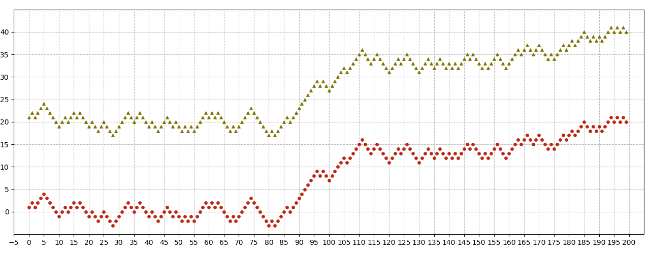
To visualize mean-centering, let’s consider two time series datasets. We can think of time-series data as $1$-dimensional, where each time step represents an observation. If two series are identical except for a difference in their $y$-intercepts (Figure $2$), we would expect them to have a correlation coefficient of $1$. Note that if their $y$-intercepts are different, their means will be proportionally different.

Figure 2: Two $1$-D time series datasets that are perfectly correlated but have different $y$-intercepts and therefore different means.

The standard mathematical way to deal with this problem is to subtract the mean from each series. To see why this works, look at what happens mathematically when one series is simply the other series with some additive offset, i.e. $\text{y}=\text{x}+\alpha$. First, let’s put the mean of $\text{y}$, ${\mu }_y$, in terms of the mean of $\text{x}$, ${\mu }_x$:

$$\begin{array}{rl}{\mu }_y& =\frac{{\sum }_i^n{x}_i+\alpha }{n}=\frac{{\sum }_i^n{x}_i}{n}+\frac{n\alpha }{n}\\ & ={\mu }_x+\alpha \end{array}$$

Now let’s compute the correlation between $\text{x}$ and $\text{y}$:

$$\begin{array}{rl}\text{corr}(\text{x},\text{y})& =\text{corr}(\text{x},\text{x}+\alpha )\\ & \\ & =\frac{\text{x}\cdot (\text{x}+\alpha )}{\Vert \text{x}{\Vert }_2\Vert \text{x}+\alpha {\Vert }_2}\\ & \\ & =\frac{{\sum }_i(x_i-{\mu }_x)(x_i+\alpha -{\mu }_y)}{\sqrt{{\sum }_i(x_i-{\mu }_x{)}^2}\sqrt{{\sum }_i(x_i+\alpha -{\mu }_y{)}^2}}\\ & \\ & =\frac{{\sum }_i(x_i-{\mu }_x)(x_i+\alpha -{\mu }_x+\alpha )}{\sqrt{{\sum }_i(x_i-{\mu }_x{)}^2}\sqrt{{\sum }_i(x_i+\alpha -{\mu }_x+\alpha {)}^2}}\\ & \\ & =\frac{{\sum }_i(x_i-{\mu }_x)(x_i-{\mu }_x)}{\sqrt{{\sum }_i(x_i-{\mu }_x{)}^2}\sqrt{{\sum }_i(x_i-{\mu }_x{)}^2}}\\ & \\ & =\text{corr}(\text{x},\text{x})\end{array}$$

In words, by subtracting the mean, we allow the series to move up or down without effecting the measure of correlation. If we had an $K$-dimensional dataset, we would subtract the means from all $K$ dimensions.

2. Scale invariance

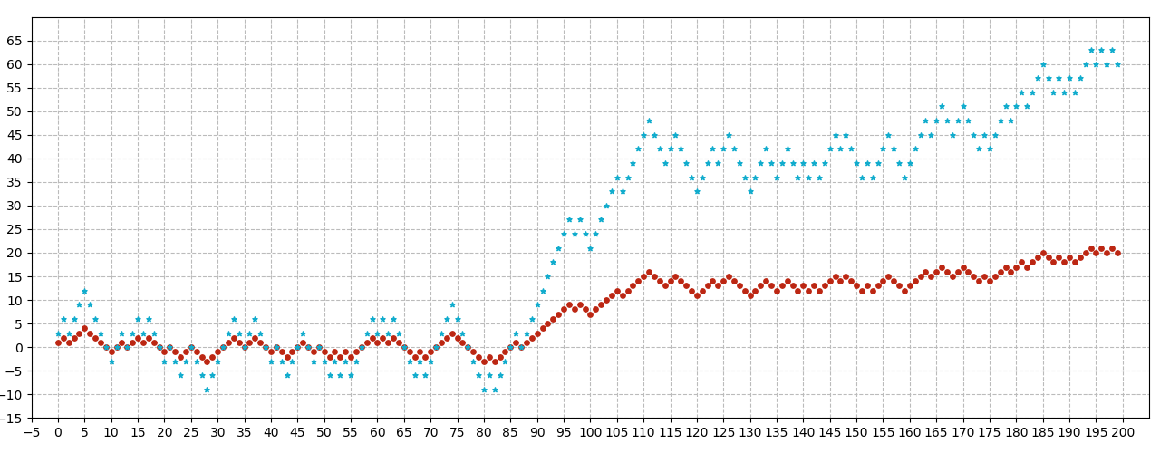
Another important property for correlation is scale invariance. This means that two variables can be perfectly correlated even though one variable changes at a scale that is disproportionate to the other. For example, the two time series in Figure $3$ are perfectly correlated.

Figure 3: Two time series that are perfectly correlated. Every value in the red time series is multiplied by $3$ to generate the blue series.

We can see this property mathematically by exploring what happens when we compute the correlation between two vectors $\text{x}$ and $\text{y}=\alpha \text{x}$ where $\alpha$ is a scalar. First, let’s again note the mean of $\text{y}$:

$${\mu }_y=\frac{{\sum }_i^n\alpha x_i}{n}=\alpha \frac{{\sum }_i^n{x}_i}{n}=\alpha {\mu }_x$$

$$\begin{array}{rl}\text{corr}(\text{x},\text{y})& =\text{corr}(\text{x},\alpha \text{x})\\ & \\ & =\frac{\text{x}\cdot (\alpha \text{x})}{\Vert \text{x}{\Vert }_2\Vert \alpha \text{x}{\Vert }_2}\\ & \\ & =\frac{{\sum }_i(x_i-{\mu }_x)(\alpha x_i-\alpha {\mu }_x)}{\sqrt{{\sum }_i(x_i-{\mu }_x{)}^2}\sqrt{{\sum }_i(\alpha x_i-\alpha {\mu }_x{)}^2}}\\ & \\ & =\frac{{\sum }_i(\alpha )(x_i-{\mu }_x)(x_i{\mu }_x)}{\sqrt{{\sum }_i(x_i-{\mu }_x{)}^2}\sqrt{{\sum }_i(\alpha {)}^2(x_i-{\mu }_x{)}^2}}\\ & \\ & =\frac{\alpha {\sum }_i(x_i-{\mu }_x)(x_i{\mu }_x)}{\alpha \sqrt{{\sum }_i(x_i-{\mu }_x{)}^2}\sqrt{{\sum }_i(x_i-{\mu }_x{)}^2}}\\ & \\ & =\frac{{\sum }_i(x_i-{\mu }_x)(x_i-{\mu }_x)}{\sqrt{{\sum }_i(x_i-{\mu }_x{)}^2}\sqrt{{\sum }_i(x_i-{\mu }_x{)}^2}}\\ & \\ & =\text{corr}(\text{x},\text{x})\end{array}$$

In words, $\text{y}$ is perfectly correlated with $\text{x}$ despite the two series being scaled differently.

3. Code

For completeness, here is the code to solve for ${\text{w}}_a$ and ${\text{w}}_b$ using Hotelling’s standard eigenvalue problem method. See my GitHub repository for a complete working version.

import numpy as np

# ------------------------------------------------------------------------------

inv  = np.linalg.inv
mm   = np.matmul

# ------------------------------------------------------------------------------

def fit_standard_eigenvalue_method(Xa, Xb):
    """
    Fits CCA parameters using the standard eigenvalue problem.
    
    :param Xa: Observations with shape (n_samps, p_dim).
    :param Xb: Observations with shape (n_samps, q_dim).
    :return:   Linear transformations Wa and Wb.
    """
    N, p = Xa.shape
    N, q = Xb.shape
    r    = min(p, q)

    Xa -= Xa.mean(axis=0)
    Xa /= Xa.std(axis=0)
    Xb -= Xb.mean(axis=0)
    Xb /= Xb.std(axis=0)

    p = Xa.shape[1]
    C   = np.cov(Xa.T, Xb.T)
    Caa = C[:p, :p]
    Cbb = C[p:, p:]
    Cab = C[:p, p:]
    Cba = C[p:, :p]

    # Either branch results in: r x r matrix where r = min(p, q).
    if q < p:
        M = mm(mm(inv(Cbb), Cba), mm(inv(Caa), Cab))
    else:
        M = mm(mm(inv(Caa), Cab), mm(inv(Cbb), Cba))

    # Solving the characteristic equation,
    #
    #     det(M - rho^2 I) = 0
    #
    # is equivalent to solving for rho^2, which are the eigenvalues of the
    # matrix.
    eigvals, eigvecs = np.linalg.eig(M)
    rhos = np.sqrt(eigvals)

    # Ensure we go through eigenvectors in descending order.
    inds    = (-rhos).argsort()
    rhos    = rhos[inds]
    eigvals = eigvals[inds]
    # NumPy returns each eigenvector as a column in a matrix.
    eigvecs = eigvecs.T[inds].T
    Wb      = eigvecs

    Wa = np.zeros((p, r))
    for i, (rho, wb_i) in enumerate(zip(rhos, Wb.T)):
        wa_i = mm(mm(inv(Caa), Cab), wb_i) / rho
        Wa[:, i] = wa_i

    # Sanity check: canonical correlations are equal to the rhos.
    Za = np.linalg.norm(mm(Xa, Wa), 2, axis=0)
    Zb = np.linalg.norm(mm(Xb, Wb), 2, axis=0)
    CCs = np.zeros(r)

    for i in range(r):
        za = Za[:, i]
        zb = Zb[:, i]
        CCs[i] = np.dot(za, zb)
    assert np.allclose(CCs, rhos)

    return Wa, Wb

Note that according to NumPy’s documentation on the eig function, eigenvalues and eigenvectors are not necessarily ordered, hence the ordering using argsort.