Simulating Geometric Brownian Motion

In mathematical finance, a standard assumption is that an asset follows a geometric Brownian motion (GBM). Formally, this means that the asset follows this stochastic differential equation (SDE):

$\text{d}S_t = \mu S_t \text{d}t + \sigma S_t \text{d}W_t, \tag{1}$

where $S_t$ is the asset price at time $t$, $\mu$ is its drift, $\sigma$ is its volatility, and $W_t$ is a Brownian motion. To rigorously understand this equation, we would need stochastic calculus in order to manipulate the stochastic differential $\text{d}W_t$, but let’s elide the technical details and focus on the discrete-time analog of this process, which I’ll write as

$\frac{\Delta S_t}{S_t} = \mu \Delta t + \sigma \sqrt{\Delta t} Z, \quad Z \sim \mathcal{N}(0, t). \tag{2}$

Here, $\Delta t$ is a discrete change in time, and $\Delta S_t$ is the change in the discrete-time process $S_t$ or

$\Delta S_t = S_{t+\Delta t} - S_t. \tag{3}$

I’ve divided both sides of the equation by $S_t$ to underscore that the SDE is modeling the relative change in the asset price (the return). For example, imagine that time is in years, and that $\Delta t$ is one day or

$\Delta t = \frac{1}{365}. \tag{4}$

Then the drift $\mu$ should the average annualized return of the asset. For example, if $\mu = 0.04$, then this means the asset’s average annualized return is $4\%$, and therefore that the daily average return is

$\mu \Delta t = \frac{4\%}{365} \approx 0.01\%. \tag{5}$

Of course, $\sigma$ should also be in annualized terms. For example, if $\sigma = 0.18$, then this means that the asset’s annualized volatility is $18\%$, and therefore that the daily volatility is

$\sigma \sqrt{\Delta t} = \frac{18\%}{\sqrt{365}} \approx 0.94\%. \tag{6}$

Here, the $\sqrt{\Delta t}$ falls naturally out of either properties of the normal distribution or the square-root of time rule, since we are assuming returns are i.i.d.

At this point, we have enough understanding to simulate the discrete-time process in Equation $2$. But a little theory will help us sanity check our results. So let’s go back to the continous-time process for a moment. A standard result is that the solution to the SDE in Equation $1$ is

$S_t = S_0 \exp\! \left\{ \left[\mu - \frac{1}{2} \sigma^2 \right] t + \sigma W_t \right\}. \tag{7}$

With a little algebra, we can easily see that this implies that the asset’s log return is normally distributed:

$\log S_t - \log S_0 \sim \mathcal{N} \! \left( \left[ \mu - \frac{1}{2}\sigma^2 \right] t, \sigma^2 t \right). \tag{8}$

Equivalently, this means that the asset price is lognormally distributed. To disambiguate the parameters of the log normal distribution from the parameters of GBM, let’s use the following notation:

$\begin{aligned} m &:= \mu - \frac{1}{2}\sigma^2, \\ s &:= \sigma. \end{aligned} \tag{9}$

(We’ll see this distinction more clearly in the simulations.) While deriving Equation $7$—technically, solving the SDE—requires stochastic calculus, the results here should make sense, since log returns approximate raw returns or

$\frac{S_{t + \Delta t} - S_t}{S_t} \approx \log S_{t + \Delta t} - \log S_t. \tag{10}$

We can see that the average raw return ($\mu$ in Equation $2$) differs from the average log return ($m$ in Equation $9$) by the adjustment factor

$-\frac{1}{2}\sigma^2. \tag{11}$

This factor arises from applying the Itô–Doeblin lemma to solve the SDE, but you can safely ignore this point if it does not make sense. Anyway, what this means is that we can simulate GBM in discrete time using Equation $2$, and then sanity check the results by confirming that over many simulations, various quantities converge to their theoretical (continuous-time) values. Let’s do that now.

Here is the basic code to simulate GBM:

# annualized drift of returns
mu = 0.04

# annualized volatility of returns
sigma = 0.18

# change in time in years
dt = 1/365

# annualized mean of log returns
m = (mu - 0.5 * sigma**2)

# annualized volatility of log returns
s = sigma

# daily log returns
logret = np.random.normal(m * dt, s * np.sqrt(dt), size=int(1/dt))

# daily raw returns
ret = np.exp(logret) - 1

# daily prices assuming S0=1
price = np.exp(logret.cumsum())

Using this code, we can simulate GBM over many trials (Figure $1$). Of course, one should do this by changing the size argument above to account for the number of trials. (Don’t write a for-loop.)

Figure 1. One thousand simulations of geometric Brownian motion using the code above. The origin line $y=0$ is drawn as a white solid line to highlight that there is indeed an empirical drift (cyan dashed line).

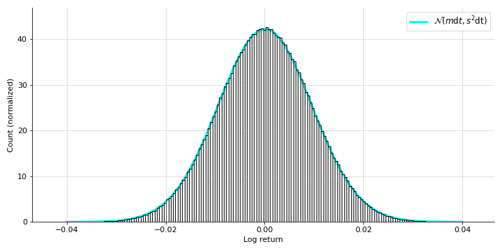
This looks directionally correct, but we can sanity check it quantitatively by comparing the simulations’ terminal distribution with the theoretical distribution (Equation $8$). Running one-hundred thousand simulations, I produced the normalized histogram in Figure $2$ and overlayed the theoretical distribution in cyan.

Figure 2. Histogram of the terminal distribution of returns over one-hundred thousand simulations.

Now from Equation $8$, we can see that the expected value of the log returns should be

$\mathbb{E}\left[\log S_{t+\Delta t} - \log S_t\right] = \left( \mu - \frac{1}{2} \sigma^2 \right) \Delta t = m \Delta t, \tag{12}$

while the expected value of the raw returns should be

$\mathbb{E}\left[\Delta S_t / S_t\right] = \mu \Delta t. \tag{13}$

We can also verify these claims quantitatively, although it’s hard to see visually with these particular numbers. For my simulations, I have the following results:

print(logrets.mean(), m * dt)
# (0.001050319587857524, 0.0010515068493150686)

print(rets.mean(), mu * dt)
# (0.0010952854516645238, 0.0010958904109589042)

And of course, we can make all our results tighter with more trials.