Log-Normal Distribution

Let $X$ be a normal random variable with mean $\mu$ and variance $\sigma^2$:

$X \sim \mathcal{N}(\mu, \sigma^2). \tag{1}$

Now define $Y$ as

$Y = \exp(X). \tag{2}$

We say that $Y$ is log-normally distributed with parameters $\mu$ and $\sigma$ or

$Y \sim \text{lognormal}(\mu, \sigma). \tag{3}$

Alternatively, we could say that $\log Y$ is normally distributed,

$\log Y \sim \mathcal{N}(\mu, \sigma^2). \tag{4}$

Let’s work through some basic properties of $Y$.

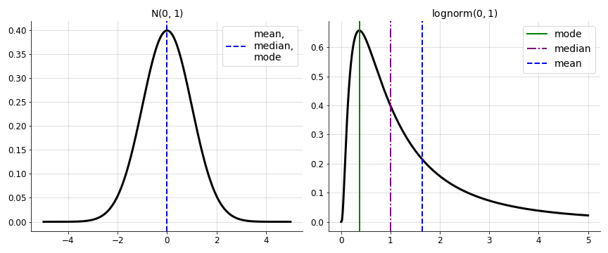
Non-negativity. Perhaps the first thing to observe is that $Y$ is a non-negative random variable (Figure $1$). This is because $e^x$ is positive for any value of $x$. Thus, the log-normal distribution often arises in cases where non-negativity is an important property of the data being modeled.

Figure 1. Normal (left) and log-normal (right) distributions, both with parameters $\mu=0$ and $\sigma=1$. The normal distribution's measures of central tendency (mean, median, mode) are all equal, while the log-normal distribution's measures are different due to the log-normal distribution's skew.

Moments. The second thing to observe is that the parameters $\mu$ and $\sigma^2$ are the mean and variance of $X$, but they are not the mean and variance of $Y$. The mean of $Y$ is

$\mathbb{E}[Y] = \mathbb{E}\left[\exp(X)\right] = \exp\left\{ \mu + \frac{1}{2} \sigma^2 \right\}. \tag{5}$

This is just a special case of the $k$-th moment of the log-normal distribution. In general, the $k$-th moment is

$\mathbb{E}[e^{Xk}] = \exp\left\{ k \mu + \frac{1}{2} k^2 \sigma^2 \right\}. \tag{6}$

See A1 for details. The variance is

$\mathbb{V}[Y] = \left(\exp\left\{\sigma^2\right\} - 1\right) \exp\left\{2\mu + \sigma^2\right\}, \tag{7}$

which can also be derived from Equation $6$. See A2 for details.

Density functions. The cumulative distribution function (CDF) of $Y$ is

$F_Y(y) = \Phi\left(\frac{\log y - \mu}{\sigma}\right), \tag{8}$

where $\Phi(x)$ is CDF of the standard normal distribution. This is trivial to derive:

$\mathbb{P}(Y \leq y) = \mathbb{P}(X \leq \log y). \tag{9}$

We can then differentiate Equation $8$ to compute the probability density function (PDF) of $Y$, which is

$f_Y(y) = \frac{1}{y \sigma \sqrt{2\pi}} \exp\left\{ -\frac{1}{2}\left[\frac{\log y - \mu}{\sigma} \right]^2 \right\}. \tag{10}$

See A3 for details.

Measures of central tendency. Using the CDF in Equation $8$, we can compute the median $m$ of $Y$, which is

$m := \exp(\mu). \tag{11}$

See A4 for details. And using the PDF in Equation $8$, we can compute the mode $d$, which is

$d := \exp(\mu - \sigma^2). \tag{12}$

See A5 for details. Given Equations $5$, $11$, and $12$, we can order these measures of central tendency as

$\exp(\mu - \sigma^2) \leq \exp(\mu) \leq \exp\!\left(\mu + \frac{1}{2} \sigma^2 \right). \tag{13}$

This tells us that a log-normal distribution’s measures are ordered left-to-right as mode, median, and then mean (Figure $1$, right).

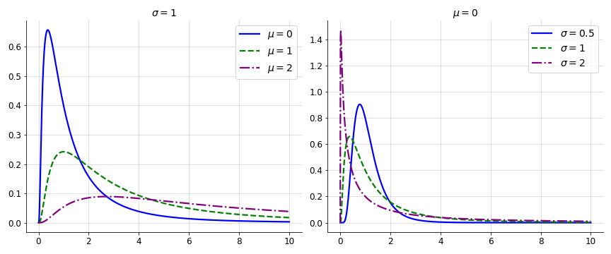
Parameterizations. Not only is $\mu$ not the mean of $Y$, it is not even a clean measure of central tendency. This is because $\mu$ is shifting $\log y$ rather than $y$. So the dispersion of $Y$ increases as either $\mu$ or $\sigma$ increases (Equation $7$ and Figure $2$).

Figure 2. Several log-normal distributions with (left) the parameter $\sigma$ fixed and (right) the parameter $\mu$ fixed. We can see that both the central tendency and dispersion of $Y$ depend on $\mu$ and $\sigma$.

Given the fact that $\mu$ and $\sigma$ are not actually the mean and standard deviations of $Y$, we can consider alternative, more natural parameterizations. One choice is to consider the exponent of each parameter, so

$\mu^* = e^{\mu}, \qquad \sigma^* = e^{\sigma}. \tag{14}$

We have already seen that $\mu^*$ is the median of $Y$, while $\sigma^*$ captures the dispersion of $Y$, although it is not the variance of $Y$.

As a final note, some statistical libraries use different parameterizations. In my mind, it is easiest to think of the “canonical” parameterization as the one used in this post and to then convert to alternative forms as needed. For an example, see A6 for details on SciPy’s parameterization of the log-normal distribution.

Appendix

A1. Moments

We want to find the $k$-th moment of $Y = e^X$ when $X \sim \mathcal{N}(\mu, \sigma^2)$. This means we want to simplify

$\mathbb{E}[Y^k] = \mathbb{E}[e^{Xk}] = \int_{-\infty}^{\infty} \exp\left\{xk\right\} \frac{1}{\sqrt{2 \pi \sigma^2}} \exp\left\{ -\frac{1}{2} \left[ \frac{x - \mu}{\sigma} \right]^2 \right\} dx. \tag{A1.1}$

We add combine the exponent terms into

$\exp\left\{ -\frac{1}{2} \left[ \frac{x - \mu}{\sigma} \right]^2 + xk\right\}. \tag{A1.2}$

Then all we need to do is simplify the expression in brackets to be again quadratic in $x$. We can then pull out any terms that do not depend on $x$, and see that the integral must be unity because probabilities are normalized. So let’s write the bracketed term as

$\begin{aligned} &-\frac{1}{2} \left[ \frac{x - \mu}{\sigma} \right]^2 + xk \\ &= -\frac{1}{2\sigma^2} \left[ x^2 - \mu^2 - 2x\mu - 2 \sigma^2 xk \right] \\ &= -\frac{1}{2\sigma^2} \left[ x^2 - \mu^2 - 2x\mu - 2 \sigma^2 xk + (2 \sigma^2 k \mu + k^2 \sigma^4) - (2 \sigma^2 k \mu + k^2 \sigma^4) \right] \\ &= -\frac{1}{2\sigma^2} \left[ (x - \mu - k \sigma^2)^2 - (2 \sigma^2 k \mu + k^2 \sigma^4) \right]. \end{aligned} \tag{A1.3}$

So we can rewrite Equation $\text{A}2$ above as

$\exp\left\{ -\frac{1}{2 \sigma^2} \left[ x - \mu - k \sigma^2 \right]^2 \right\} \exp\left\{ k \mu + \frac{1}{2} k^2 \sigma^2 \right\}. \tag{A1.4}$

The right term does not depend on $x$ and can thus be pulled out the integral, giving us

$\mathbb{E}[e^{Xk}] = \exp\left\{ k \mu + \frac{1}{2} k^2 \sigma^2 \right\} \int_{-\infty}^{\infty} \frac{1}{\sqrt{2 \pi \sigma^2}} \exp\left\{ -\frac{1}{2 \sigma^2} \left[ x - \mu - k \sigma^2 \right]^2 \right\} dx. \tag{A1.5}$

The integral must be equal to unity and therefore

$\mathbb{E}[e^{Xk}] = \exp\left\{ k \mu + \frac{1}{2} k^2 \sigma^2 \right\}. \tag{A1.6}$

We can easily compute the mean and variance of $X$ using Equation $A6$.

A2. Variance

Using A1, we can see that the variance of $Y$ is

$\begin{aligned} \mathbb{V}[Y] &= \mathbb{E}[Y^2] - \mathbb{E}[Y]^2 \\ &= \exp\left\{ 2\mu + 2\sigma^2 \right\} - \left[ \exp\left\{ \mu + \frac{1}{2}\sigma^2 \right\} \right]^2 \\ &= \exp\left\{ \sigma^2 - 1 \right\} \exp\left\{ 2 \mu + \sigma^2 \right\}. \end{aligned} \tag{A2.1}$

And we’re done.

A3. Probability density function

Let $\Phi(x)$ and $\varphi(x)$ denote the CDF and PDF of $X$ respectively. Then the PDF of $Y$ is

$\begin{aligned} f_Y(y) &= \frac{d}{dy}\mathbb{P}(Y \leq y) \\ &= \frac{d}{dy} \mathbb{P}(X \leq \log y) \\ &= \frac{d}{dy} \Phi \! \left( \frac{\log y - \mu}{\sigma} \right) \\ &= \varphi \! \left( \frac{\log y - \mu}{\sigma} \right) \frac{d}{dy} \! \left( \frac{\log y - \mu}{\sigma} \right) \\ &= \varphi \! \left( \frac{\log y - \mu}{\sigma} \right) \! \frac{1}{y \sigma}. \end{aligned} \tag{A3.1}$

Using the definition of $\varphi(x)$, we have

$f_Y(y) = \frac{1}{y \sigma \sqrt{2\pi}} \exp\left\{ -\frac{1}{2}\left[\frac{\log y - \mu}{\sigma} \right]^2 \right\}, \tag{A3.2}$

as desired.

A4. Median

The median $m$ of a random variable is a constant such that

$\mathbb{P}\left(-\infty \leq Y \leq m\right) = \mathbb{P}\left(m \leq Y \leq \infty \right). \tag{A4.1}$

In words, half of the probability is on either side of $m$. We can see that in the case that $Y$ is log-normally distributed, we have

$\begin{aligned} \mathbb{P}\left(-\infty \leq \exp X \leq m\right) &= \mathbb{P}\left( m \leq \exp X \leq \infty\right) \\ &\Downarrow \\ \mathbb{P}\left(-\infty \leq X \leq \log m\right) &= \mathbb{P}\left( \log m \leq X \leq \infty\right). \end{aligned} \tag{A4.2}$

But for $X$, the median is $\mu$, and therefore we have $\mu = \log m$, which implies that $m = \exp \mu$, as desired.

A5. Mode

To compute the mode $d$ of a distribution, we want to compute

$d := y^{\star} = \arg\!\max_{y} f_Y(y). \tag{A5.1}$

To compute this, we take the derivative of the PDF, set it equal to zero, and solve for $y$. In addition, we should confirm that $m$ is the local maximum using a second derivative test.

The first derivative is

$\begin{aligned} f^{\prime}_Y(y) &= \left[ -\frac{e^{-1/2 ((\log y - \mu) / \sigma)^2}}{y^2 \sigma \sqrt{2\pi}} + \frac{e^{-1/2 ((\log y - \mu) / \sigma)^2}}{y \sigma \sqrt{2\pi}} \left(\frac{\mu - \log y}{\sigma}\right) \frac{1}{y \sigma} \right] \\ &= \frac{1}{y^2 \sigma \sqrt{2 \pi}} e^{-1/2 ((\log y - \mu) / \sigma)^2} \left[1 + \frac{\log y - \mu}{\sigma^2}\right]. \end{aligned} \tag{A5.2}$

Let’s set this equal to zero and solve for $y$:

$\begin{aligned} 0 &= \frac{1}{y^2 \sigma \sqrt{2 \pi}} e^{-1/2 ((\log y - \mu) / \sigma)^2} \left[1 + \frac{\log y - \mu}{\sigma^2}\right] \\ &= 1 + \frac{\log y - \mu}{\sigma^2} \\ -\sigma^2 + \mu &= \log y \\ &\Downarrow \\ y &= \exp(\mu - \sigma^2). \end{aligned} \tag{A5.3}$

We should confirm this is a maximum with a second derivative test. However, I don’t want to take the derivative of Equation $\text{A}5.2$. See the Book of Statistical Proofs for a complete proof.

A6. SciPy

SciPy uses a parameter s for $\sigma$ and a parameter scale for $\exp \mu$. This is a SciPy convention in which multiple distributions use the same parameter names (loc, shape, scale, …). Since $\mu$ is not strictly a location parameter—it also affects the dispersion—we can only specify $\mu$ a la Equation $3$ using the median $\exp \mu$. I am not sure why the argument for $\sigma$ is named s rather than shape.

Here is a sanity check,

from scipy.stats import lognorm

mu = 2
sigma = 0.7
m, v = lognorm(scale=np.exp(mu), s=sigma).stats(moments="mv")

print(np.exp(mu + 0.5 * sigma**2))
# 9.440415556460355
print(m.item())
# 9.440415556460353

print((np.exp(sigma**2) - 1) * np.exp(2 * mu + sigma**2))
# 56.352935774951334
print(v.item())
# 56.35293577495132

which confirms our understanding of the parameterization.