Bienaymé's Identity

Let $B_n$ denote a random variable which is itself the sum of $n$ random variables,

$B_n := \sum_{i=1}^n X_i. \tag{1}$

Bienaymé’s identity, named after the French statistician Irénée-Jules Bienaymé, states that the variance of $B_n$ is

$\mathbb{V}[B_n] = \sum_{i=1}^n \mathbb{V}[X_i] \; + \!\!\! \sum_{i,j=1,i \neq j}^n \!\!\!\! \text{cov}\left[X_i, X_j \right]. \tag{2}$

If we think of variance as simply a special case of covariance, since

$\mathbb{V}[X_i] = \text{cov}\left[X_i, X_i\right], \tag{3}$

then we can write Equation $2$ as

$\mathbb{V}[B_n] = \! \sum_{i,j=1}^n \text{cov}\left[X_i, X_j \right]. \tag{4}$

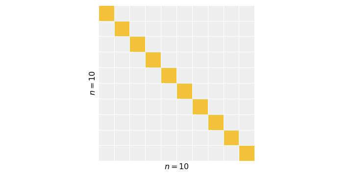
In either case, we can visualize this identity as summing the elements of the covariance matrix of the vector $[X_1, \dots, X_n]$ (Figure $1$). In Equation $2$, we break the sum into the diagonal and off-diagonal elements, while in Equation $4$, we denote the diagonal elements with the same notation as the off-diagonal elements.

Figure 1. Visualization of Bienaymé's identity. The matrix represents an $n \times n$ covariance matrix of the vector $[X_1, \dots, X_n]$. The variances or diagonal elements (gold) are captured in the middle sum in Equation $2$, while the covariances or off-diagonal elements (gray) are captured in the right sum in Equation $2$.

If we write the covariance in terms of Pearson’s correlation coefficient $\rho$, then the identity in Equation $3$ becomes

$\mathbb{V} [B_n] = \!\! \sum_{i,j=1}^n \rho_{ij} \; \sqrt{\mathbb{V}[X_i] \mathbb{V}[X_j]}. \tag{5}$

An important special case of Bienaymé’s identity is when the random variables are independent or uncorrelated ($\rho = 0$). In either case, the covariance between the random variables is zero or

$\text{cov}\left[X_i, X_j\right] = 0, \quad i \neq j. \tag{6}$

And so clearly, we have

$\mathbb{V} [B_n] = \sum_{i=1}^n \mathbb{V}[X_i]. \tag{7}$

This leads to rules such as the square root of time rule or adages such as “variances add”.

With a little thought, Bienaymé’s identity is fairly intuitive. If we add random variables together, then we are compounding uncertainty. However, that uncertainty is less if the elements are independent or uncorrelated, in which case their uncertainty is unrelated. But in the worst case, all random variables are highly correlated with $\rho = 1$, which maximizes the variance of $B_n$. Alternatively, in the best case, all random variables are highly anti-correlated with $\rho = -1$, which minimizes the variance of $B_n$.

Finally, proving Bienaymé’s identity really amounts to understanding how to square a sum of terms. In general, it is true that

$\left( a_1 + a_2 + \dots + a_k \right)^2 = \sum_{i=1}^k a_i^2 + \!\!\! \sum_{i,j=1, i\neq j}^k \!\! a_i a_j. \tag{8}$

We can see that this is true with a simple proof:

$\begin{aligned} \left( \sum_{i=1}^k a_i \right)^2 &= \left( \sum_{i=1}^k a_i \right) \left( \sum_{j=1}^k a_j \right) \\ &= \sum_{i=1}^k \sum_{j=1}^k a_i a_j \\ &= \sum_{i=1}^k a_i^2 + \!\!\! \sum_{i,j=1, i\neq j}^n \!\! a_i a_j. \end{aligned} \tag{9}$

We can then apply Equation $8$ twice and consolidate terms to derive Bienaymé’s identity,

$\begin{aligned} \mathbb{V}[B_n] &= \mathbb{E}\left[(B_n + \mathbb{E}\left[B_n\right])^2\right] \\ &= \mathbb{E}\left[B_n^2\right] - \mathbb{E}\left[B_n\right]^2 \\ &= \mathbb{E}\left[(X_1 + \dots + X_n)^2\right] - \mathbb{E}\left[X_1 + \dots + X_n \right]^2 \\ &= \mathbb{E} \left[ \sum_{i=1}^n X_i^2 + \!\!\! \sum_{i,j=1, i\neq j}^n \!\!\! X_i X_j \right] - \left[ \sum_{i=1}^n \mathbb{E}[X_i]^2 + \!\!\! \sum_{i,j=1, i\neq j}^n \!\! \mathbb{E}[X_i] \mathbb{E}[X_j] \right] \\ &= \sum_{i=1}^n \mathbb{E} \left[ X_i^2 \right] + \!\!\! \sum_{i,j=1, i\neq j}^n \!\!\! \mathbb{E} \left[ X_i X_j \right] - \sum_{i=1}^n \mathbb{E}[X_i]^2 - \!\!\! \sum_{i,j=1, i\neq j}^n \!\!\! \mathbb{E}[X_i] \mathbb{E}[X_j] \\ &= \sum_{i=1}^n \left[ \mathbb{E} \left[ X_i^2 \right] + \mathbb{E}[X_i]^2 \right] + \!\!\! \sum_{i,j=1, i\neq j}^n \!\!\! \left[ \mathbb{E} \left[ X_i X_j \right] - \mathbb{E}[X_i] \mathbb{E}[X_j] \right], \tag{10} \end{aligned}$

as desired.