High-Dimensional Variance

When $X$ is a random scalar, we call $\mathbb{V}[X]$ the variance of $X$, and define it as the average squared distance from the mean:

$\mathbb{V}[X] := \sigma^2 = \mathbb{E}\!\left[\left(X - \mathbb{E}[X]\right)^2\right]. \tag{1}$

The mean $\mathbb{E}[X]$ is a measure of the central tendency of $X$, while the variance $\mathbb{V}[X]$ is a measure of the dispersion about this mean. Both metrics are moments of the distribution.

However, when $\mathbf{X}$ is a random vector or an ordered list of random scalars

$\mathbf{X} = \begin{bmatrix} X_1 \\ X_2 \\ \vdots \\ X_n \end{bmatrix}, \tag{2}$

then, at least in my experience, people do not talk about the variance of $\mathbf{X}$; rather, they talk about the covariance matrix of $\mathbf{X}$, denoted $\text{cov}[\mathbf{X}]$:

$\text{cov}[\mathbf{X}] := \boldsymbol{\Sigma} = \mathbb{E}\!\left[\left(\mathbf{X} - \mathbb{E}[\mathbf{X}])(\mathbf{X} - \mathbb{E}[\mathbf{X}]\right)^{\top}\right]. \tag{3}$

Now Equations $1$ and $3$ look quite similar, and I think it is natural to eventually ask: is a covariance matrix just a high- or multi-dimensional variance of $\mathbf{X}$? Does this notation and nomenclature make sense?

$\mathbb{V}[\mathbf{X}] := \text{cov}[\mathbf{X}]. \tag{4}$

Of course, this is not my idea, but this was not how I was taught to think about covariance matrices. But I think it is an illuminating connection. So let’s explore this idea that a covariance matrix is just high-dimensional variance.

Definitions

To start, it is clear from definitions that a covariance matrix is related variance. We can write the outer product in Equation $3$ explicitly as:

$\boldsymbol{\Sigma} = \begin{bmatrix} \mathbb{E}[(X_1 - \mathbb{E}[X_1])(X_1 - \mathbb{E}[X_1])] & \dots & \mathbb{E}[(X_1 - \mathbb{E}[X_1])(X_n - \mathbb{E}[X_n])] \\ \vdots & \ddots & \vdots \\ \mathbb{E}[(X_n - \mathbb{E}[X_n])(X_1 - \mathbb{E}[X_1])] & \dots & \mathbb{E}[(X_n - \mathbb{E}[X_n])(X_n - \mathbb{E}[X_n])] \end{bmatrix}. \tag{5}$

Clearly the diagonal elements in $\boldsymbol{\Sigma}$ are the variances of the scalars $X_i$. So $\text{cov}[\mathbf{X}]$ still captures the dispersion of each $X_i$.

But what are the cross-terms? These are the covariances of the pairwise combinations of $X_i$ and $X_j$, defined as

$\sigma_{ij} := \text{cov}(X_i, X_j) = \mathbb{E}[(X_i - \mathbb{E}[X_i])(X_j - \mathbb{E}[X_j])]. \tag{6}$

An obvious observation is that Equation $6$ is a generalization of Equation $1$. Thus, variance ($i=j$) is simply a special case of covariance:

$\mathbb{V}[X_i] = \text{cov}(X_i, X_i). \tag{7}$

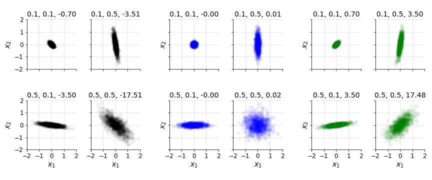
Furthermore, we can see that $\sigma_{ij}$ is not just a function of the univariate variance of each random variable; it is also a function of whether the two variances are correlated with the other. As a simple thought experiment, imagine that $X_i$ and $X_j$ both had high variances but were uncorrelated with each other, meaning that there was no relationship between large (small) values of $X_i$ and large (small) values of $X_j$. Then we would still expct $\sigma_{ij}$ to be small (Figure $1$).

Figure 1. Empirical distributions of two random variables $X_1$ and $X_2$. Each subplot is labeled with three numbers representing $\sigma_1$, $\sigma_2$ and $\sigma_{12}$ respectively. (Black subplots) $X_1$ and $X_2$ are negatively correlated with Pearson correlation coefficient $\rho = -0.7$. (Blue subplots) $X_1$ and $X_2$ are uncorrelated. (Green subplots) $X_1$ and $X_2$ are postively correlated ($\rho = 0.7$).

This is the intuitive reason that $\sigma_{ij}$ can be written in terms of the Pearson correlation coefficient $\rho_{ij}$:

$\sigma_{ij} = \rho_{ij} \sigma_i \sigma_j. \tag{8}$

Again, this generalizes Equation $1$ but with $\rho_{ii} = 1$.

Using the $\sigma_{ij}$ notation from Equations $8$ we can rewrite the covariance matrix as

$\boldsymbol{\Sigma} = \begin{bmatrix} \sigma_1^2 & \rho_{12} \sigma_1 \sigma_2 & \dots & \rho_{1n} \sigma_1 \sigma_n \\ \rho_{21} \sigma_2 \sigma_1 & \sigma_2^2 & \dots & \rho_{2n} \sigma_2 \sigma_n \\ \vdots & \ddots & \vdots \\ \rho_{n1} \sigma_n \sigma_1 & \rho_{n2} \sigma_2 \sigma_n & \dots & \sigma_n^2 \end{bmatrix}. \tag{9}$

And with a little algebra, we can decompose the matrix in Equation $9$ into a form that looks strikingly like a multi-dimensional Equation $8$:

$\boldsymbol{\Sigma} = \begin{bmatrix} \sigma_1 & & & \\ & \sigma_2 & & \\ & & \ddots & \\ & & & \sigma_n \end{bmatrix} \begin{bmatrix} 1 & \rho_{12} & \dots & \rho_{1n} \\ \rho_{21} & 1 & \dots & \rho_{2n} \\ \vdots & \vdots & \ddots & \vdots \\ \rho_{n1} & \rho_{n2} & \dots & 1 \end{bmatrix} \begin{bmatrix} \sigma_1 & & & \\ & \sigma_2 & & \\ & & \ddots & \\ & & & \sigma_n \end{bmatrix}. \tag{10}$

The middle matrix is correlation matrix, which captures the Pearson (linear) correlation between all the variables in $\mathbf{X}$. So a covariance matrix of $\mathbf{X}$ captures both the dispersion of each $X_i$ and how it covaries with the other random variables. If we think of scalar variance as a univariate covariance matrix, then one-dimensional case can be written as

$\boldsymbol{\Sigma} = \begin{bmatrix} \text{cov}(X, X) \end{bmatrix} = \begin{bmatrix} \sigma \end{bmatrix} \begin{bmatrix} 1 \end{bmatrix} \begin{bmatrix} \sigma \end{bmatrix}. \tag{11}$

Equation $11$ is not useful from a practical point of view, but in my mind, it underscores the view that univariate variance is a special case of covariance (matrices).

Finally, note that Equation $10$ gives us a useful way to compute the correlation matrix $\mathbf{C}$ from the covariance matrix $\boldsymbol{\Sigma}$. It is

$\mathbf{C} := \begin{bmatrix} 1/ \sigma_1 & & \\ & \ddots & \\ & & 1 / \sigma_n \end{bmatrix} \boldsymbol{\Sigma} \begin{bmatrix} 1 / \sigma_1 & & \\ & \ddots & \\ & & 1 / \sigma_n \end{bmatrix}. \tag{12}$

This is because the inverse of a diagonal matrix is simply the reciprocal of each element along the diagonal.

Properties

Some important properties of univariate variance have multidimensional analogs. For example, let $a$ be a non-random number. Recall that the variance of $a X$ scales with $a^2$ or that

$\mathbb{V}[a X] = a^2 \mathbb{V}[X] = a^2 \sigma^2. \tag{13}$

And in the general case, $a$ is a non-random matrix $\mathbf{A}$ and

$\begin{aligned} \mathbb{V}[\mathbf{A} \mathbf{X}] &= \mathbf{A}^{\top} \boldsymbol{\Sigma} \mathbf{A} \\ &= \mathbb{E}\!\left[\left(\mathbf{AX} - \mathbb{E}[\mathbf{AX}])(\mathbf{AX} - \mathbb{E}[\mathbf{AX}]\right)^{\top}\right] \\ &= \mathbf{A} \mathbb{E}\!\left[\left(\mathbf{X} - \mathbb{E}[\mathbf{X}])(\mathbf{X} - \mathbb{E}[\mathbf{X}]\right)^{\top} \right] \mathbf{A}^{\top} \\ &= \mathbf{A} \boldsymbol{\Sigma} \mathbf{A}^{\top}. \end{aligned} \tag{14}$

So both $\mathbb{V}[X]$ and $\mathbb{V}[\mathbf{X}]$ are quadratic with respect to multiplicative constants!

As a second example, recall that the univariate variance of $a + X$ is just the variance of $X$:

$\mathbb{V}[a + X] = \mathbb{V}[X]. \tag{15}$

This is intuitive. A constant shift in the distribution does not change its dispersion. And again, in the general case, a constant shift in a multivariate distribution does not change its dispersion:

$\begin{aligned} \mathbb{V}[\mathbf{A} + \mathbf{X}] &= \mathbb{E}\!\left[\left(\mathbf{A} + \mathbf{X} - \mathbb{E}[\mathbf{A} + \mathbf{X}])(\mathbf{A} + \mathbf{X} - \mathbb{E}[\mathbf{A} + \mathbf{X}]\right)^{\top}\right] \\ &= \mathbb{E}\!\left[\left(\mathbf{X} - \mathbb{E}[\mathbf{X}])(\mathbf{X} - \mathbb{E}[\mathbf{X}]\right)^{\top} \right] \\ &= \boldsymbol{\Sigma}. \end{aligned} \tag{16}$

Finally, a standard decomposition of variance is to write it as

$\mathbb{V}[X] = \mathbb{E}[X^2] - \mathbb{E}[X]^2. \tag{17}$

And this standard decomposition has a multi-dimensional analog:

$\begin{aligned} \mathbb{V}[\mathbf{X}] &= \mathbb{E}\!\left[\left(\mathbf{X} - \mathbb{E}[\mathbf{X}])(\mathbf{X} - \mathbb{E}[\mathbf{X}]\right)^{\top}\right] \\ &= \mathbb{E}\!\left[ \mathbf{X}\mathbf{X}^{\top} - 2 \mathbb{E}[\mathbf{X}] \mathbf{X}^{\top} + \mathbb{E}[\mathbf{X}] \mathbb{E}[\mathbf{X}]^{\top} \right] \\ &= \mathbb{E}[\mathbf{X}\mathbf{X}^{\top}] - \mathbb{E}[\mathbf{X}] \mathbb{E}[\mathbf{X}]^{\top}. \end{aligned} \tag{18}$

Anyway, my point is not to provide detailed or comprehensive proofs, but only to underscore that covariance matrices have properties that indicate they are simply high-dimensional (co)variances.

Non-negativity

Another neat connection is that covariance matrices are positive semi-definite (PSD), which I’ll denote with

$\mathbb{V}[\mathbf{X}] = \boldsymbol{\Sigma} \succeq 0, \tag{19}$

while univariate variances are non-negative numbers:

$\mathbb{V}[X] = \sigma^2 \geq 0. \tag{20}$

In this view, the Cholesky decomposition of a PSD matrix is simply a high-dimensional square root! So the Cholesky factor $\mathbf{L}$ can be viewed as the high-dimensional standard deviation of $X$, since

$\boldsymbol{\Sigma} = \mathbf{L}\mathbf{L}^{\top} \quad\implies\quad \mathbf{L} \approx \sigma. \tag{21}$

Here, I am wildly abusing notation to use $\approx$ to mean “analogous to”.

Precision and whitening

The precision of a scalar random variable is the reciprocal of its variance:

$p = \frac{1}{\sigma^2}. \tag{22}$

Hopefully the name is somewhat intuitive. When a random variable has high precision, this means it has low variance and thus a smaller range of possible outcomes. A common place that precision arises is when whitening data, or standardizing it to have zero mean and unit variance. We can do this by subtracting the mean of $X$ and then dividing it by its standard deviation:

$Z = \frac{X - \mathbb{E}[X]}{\sigma}. \tag{23}$

This is sometimes referred to as z-scoring.

What’s the multivariate analog to this? We can define the precision matrix $\mathbf{P}$ as the inverse of the covariance matrix or

$\mathbf{P} = \boldsymbol{\Sigma}^{-1}. \tag{24}$

Given the Cholesky decomposition in Equation $21$ above, we can compute the Cholesky factor of the precision matrix as:

$\begin{aligned} \mathbf{P} &= \left( \mathbf{L}\mathbf{L}^{\top} \right)^{-1} \\ &= \left( \mathbf{L}^{\top} \right)^{-1} \mathbf{L}^{-1} \\ &= \left( \mathbf{L}^{-1} \right)^{\top} \mathbf{L}^{-1}. \end{aligned} \tag{25}$

So the multivariate analog to Equation $23$ is

$\mathbf{Z} = \mathbf{L}^{-1} \left( \mathbf{X} - \mathbb{E}[\mathbf{X}] \right). \tag{26}$

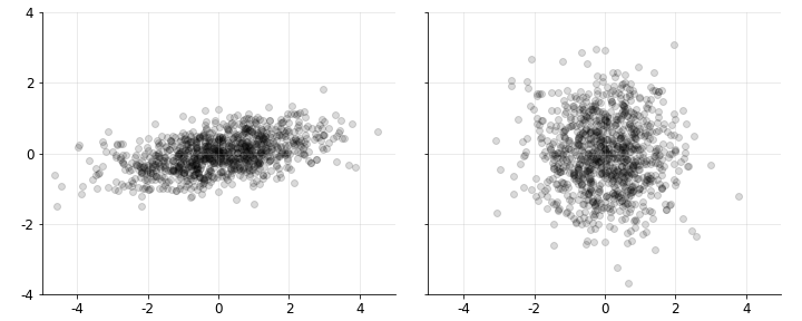
The geometric or visual effect of this operation is to apply a linear transformation (rotation) of our data (samples of the random vector) with covariance matrix $\boldsymbol{\Sigma}$ into a new set of variables with an identity covariance matrix (Figure $2$).

Figure 2. (Left) Samples of a random variable $\mathbf{X}$ with variances $\sigma_1 = 1.5$ and $\sigma_2 = 0.5$ and correlation $\rho = 0.5$. (Right) Samples rotated by the Cholesky factor of the known covariance matrix, as in Equation $26$. The effect is that the rotated samples are uncorrelated with unit variances.

Ignoring the mean, we can easily verify this transformation works:

$\begin{aligned} \mathbb{V}[\mathbf{Z}] &= \mathbb{E}[(\mathbf{L}^{-1}\mathbf{X})(\mathbf{L}^{-1}\mathbf{X})^{\top}] \\ &= \mathbb{E}[\mathbf{L}^{-1} \mathbf{X} \mathbf{X}^{\top} (\mathbf{L}^{-1})^{\top}] \\ &= \mathbf{L}^{-1} \mathbb{E}[\mathbf{X} \mathbf{X}^{\top}] (\mathbf{L}^{-1})^{\top} \\ &= \mathbf{L}^{-1} \boldsymbol{\Sigma} (\mathbf{L}^{\top})^{-1} \\ &= \mathbf{I}. \end{aligned} \tag{27}$

This derivation is a little more tedious with a mean, but hopefully the idea is clear. Why the Cholesky decomposition actually works is a deeper idea, one worth its own post, but I think the essential ideas are also captured in principal components analysis (PCA).

Summary statistics

It would be useful to summarize the information in a covariance matrix with a single number. To my knowledge, there are at least two such summary statistics that capture different types of information.

Total variance. The total variance of a random vector $\mathbf{X}$ is the trace of its covariance matrix or

$\sigma^2_{\text{tv}} := \text{tr}\left(\boldsymbol{\Sigma}\right) = \sum_{i=1}^n \sigma_i^2. \tag{28}$

We can see that total variance is a scalar that summarizes the variance across the components of $\mathbf{X}$. This concept is used in PCA, where total variance is preserved across the transformation. Of course, in the one-dimensional case, total variance is simply variance, $\sigma^2_{\text{tv}} = \sigma^2$.

Generalized variance. The generalized variance (Wilks, 1932) of a random vector $\mathbf{X}$ is the determinant of its covariance matrix or

$\sigma^2_{\text{gv}} := \text{det}(\boldsymbol{\Sigma}) = | \boldsymbol{\Sigma} |. \tag{29}$

There are nice geometric interpretations of the determinant, but perhaps the simplest way to think about it here is that the determinant is equal to the product of the eigenvalues of $\boldsymbol{\Sigma}$ or

$| \boldsymbol{\Sigma} | = \prod_{i=1}^n \lambda_i. \tag{30}$

So we can think of generalized variance as capturing the magnitude of the linear transformation represented by $\boldsymbol{\Sigma}$.

Generalized variance is quite different from total variance. For example, consider the two-dimensional covariance matrix implied by the following values:

$\sigma_1 = \sigma_2 = \rho = 1. \tag{31}$

Clearly, the total variance is two, while the determinant is one. Now imagine that the variables are highly correlated, that $\rho = 0.98$. Then the total variance is still two, but the determinant is now smaller, as the matrix becomes “more singular” (it is roughly $0.039$). So total variance, as its name suggests, really just summarizes the dispersion in $\boldsymbol{\Sigma}$, while generalized variance also captures how the variables in $\mathbf{X}$ covary. When the variables in $\mathbf{X}$ are highly (un-) correlated, generalized variance will be low (high).

Examples

Let’s end with two illuminating examples that use the ideas in this post.

Multivariate normal. First, recall that the probability density function (PDF) for a standard normal random variable is

$p(x; \mu, \sigma^2) = \frac{1}{\sqrt{2\pi} \sigma} \exp\left\{ -\frac{1}{2} \left( \frac{x - \mu}{\sigma} \right)^2 \right\}. \tag{32}$

We can immediately see that the squared term is just the square of Equation $23$. Now armed with the interpretation that a covariance matrix is high-dimensional variance, consider the PDF for a multivariate normal random variable:

$p(\mathbf{x}; \boldsymbol{\mu}, \boldsymbol{\Sigma}) = \frac{1}{(2\pi)^{-n/2} |\boldsymbol{\Sigma}|^{-1/2}} \exp\left\{ -\frac{1}{2} \left( \mathbf{x} - \boldsymbol{\mu} \right)^{\top} \boldsymbol{\Sigma}^{-1} \left( \mathbf{x} - \boldsymbol{\mu} \right) \right\}. \tag{33}$

We can see that the Mahalanobis distance is a multivariate whitening. And the variance is the normalizing term,

$\frac{1}{\sqrt{2 \pi} \sigma} \tag{34}$

has a multivariate analog that is generalized variance above.

Correlated random variables. Consider a scalar random variable $Z$ with unit variance, $\mathbb{V}[Z] = 1$. We can transform this into a random variable $X$ with variance $\sigma^2$ by multiplying $Z$ by $\sigma$:

$\mathbb{V}[\sigma Z] = \sigma^2 \mathbb{V}[{Z}] = \sigma^2. \tag{35}$

What is the multi-dimensional version of this? If we have two random variables

$\mathbf{Z} = \begin{bmatrix}Z_1 \\ Z_2\end{bmatrix}, \tag{36}$

how can we transform them into a random variable $\mathbf{X}$ with covariance matrix $\boldsymbol{\Sigma}$? Clearly, we multiply $\mathbf{Z}$ by the Cholesky factor, a la Equation $26$.

What this suggests, however, is a generic algorithm for generating correlated random variables: we multiply $\mathbf{Z}$ by the Cholesky factor of the covariance matrix when $\sigma_1 = \dots = \sigma_n = 1$. In the two-by-two case, that’s

$\text{cholesky}\left(\begin{bmatrix} 1 & \rho \\ \rho & 1 \end{bmatrix}\right) = \mathbf{L} \mathbf{L}^{\top} = \begin{bmatrix} 1 & 0 \\ \rho & \sqrt{1 - \rho^2} \end{bmatrix} \begin{bmatrix} 1 & \rho \\ 0 & \sqrt{1 - \rho^2} \end{bmatrix} \tag{37}$

This suggests that an algorithm: draw two i.i.d. random variables $Z_1$ and $Z_2$, both with unit variance. Then set

$\begin{aligned} X_1 &:= Z_1 \\ X_1 &:= Z_1 \rho + Z_2 \sqrt{1 - \rho^2}. \end{aligned} \tag{38}$

Of course, this is nice because it can be vectorized and extends to an arbitrary number of random variables. And we can easily account for non-unit variances if we would like.

Conclusion

With the proper framing, it is fairly natural to think of $\boldsymbol{\Sigma}$ as simply variance and to denote it as $\mathbb{V}[\mathbf{X}]$. This framing is useful because makes certain properties of covariance matrices almost obvious, such as why they are positive semi-definiteness or why their inverses appear when whitening data. However, high-dimensional variance has properties that are not important in one-dimension, such as the correlation between the variables in $\mathbf{X}$. Thus in my mind, the best framing is that univariate variance is really a special case of covariance matrices. However, in my mind, either reframing is useful for gaining a deeper intuition for the material.