Simple Linear Regression and Correlation

Consider simple linear regression or linear regression with a single independent variable,

$y_n = \alpha + \beta x_n + \varepsilon_n. \tag{1}$

$\beta$ is the model’s slope, and $\alpha$ is the model’s intercept. There is an interesting relationship between the estimated linear coefficient $\hat{\beta}$ and Pearson’s correlation coefficient between the predictors and targets, $\rho_{xy}$. The goal of this post is to understand this relationship better.

Univariate normal equation

Let’s rederive the normal equations for ordinary least squares (OLS), which minimizes the sum of squared residuals:

$\begin{aligned} J(\beta, \alpha) &= \sum_{n=1}^N (y_n - \alpha - \beta x_n)^2, \\ \hat{\alpha}, \hat{\beta} &= \arg\!\min_{\alpha, \beta} J(\beta, \alpha). \end{aligned} \tag{2}$

We can find the minimizers for $\beta$ and $\alpha$ by differentiating $J$ w.r.t. these parameters and solving for them after setting the derivative equal to zero. (We are ignoring the endpoints and second-order conditions since this is an established result.)

First, let’s solve for intercept $\alpha$. We take the derivative of the objective function w.r.t. to $\alpha$,

$\begin{aligned} \frac{d J}{d \alpha} &= \sum_{n=1}^N \frac{d}{d \alpha} (y_n - \alpha - \beta x_n)^2 \\ &= \sum_{n=1}^N 2 (y_n - \alpha - \beta x_n) (- 1) \\ &= 2 \left( \sum_{n=1}^N \beta x_n - y_n + \alpha \right), \end{aligned} \tag{3}$

set this equal to zero, and then solve for $\alpha$:

$\begin{aligned} 0 &= 2 \left( \sum_{n=1}^N \beta x_n - \sum_{n=1}^N y_n + N \alpha \right), \\ &\Downarrow \\ \hat{\alpha} &= \bar{y} - \beta \bar{x}, \end{aligned} \tag{4}$

where $\bar{x}$ and $\bar{y}$ are the sample means, e.g. $\bar{x} = (1/N) \sum_{n=1}^N x_n$.

Next, let’s solve for the slope $\beta$. We take the derivative of our objective function w.r.t. $\beta$,

$\begin{aligned} \frac{d J}{d \beta} &= \sum_{n=1}^N \frac{d}{d \beta} (y_n - \alpha - \beta x_n)^2 \\ &= \sum_{n=1}^N 2 (y_n - \alpha - \beta x_n) (- x_n) \\ &= 2 \left( \sum_{n=1}^N \beta x_n^2 - x_n y_n + \alpha x_n \right), \end{aligned} \tag{5}$

set this equal to zero, and solve, plugging in the value of $\alpha$ that we just computed:

$\begin{aligned} 0 &= 2 \left[ \sum_{n=1}^N \beta x_n^2 - x_n y_n + \alpha x_n \right], \\ &\Downarrow \\ \alpha \sum_{n=1}^N x_n + \beta \sum_{n=1}^N x_n^2 &= \sum_{n=1}^N x_n y_n \\ (\bar{y} - \bar{x} \beta) \sum_{n=1}^N x_n + \beta \sum_{n=1}^N x_n^2 &= \sum_{n=1}^N x_n y_n \\ \bar{y} \sum_{n=1}^N x_n - \bar{x} \beta \sum_{n=1}^N x_n + \beta \sum_{n=1}^N x_n^2 &= \sum_{n=1}^N x_n y_n \\ \beta \left[ \sum_{n=1}^N x_n^2 - \frac{1}{N} \sum_{n=1}^N x_n \sum_{n=1}^N x_n \right] &= \sum_{n=1}^N x_n y_n - \frac{1}{N} \sum_{n=1}^N y_n \sum_{n=1}^N x_n . \end{aligned} \tag{6}$

To summarize, the OLS estimates for $\hat{\alpha}$ and $\hat{\beta}$ are

$\begin{aligned} \hat{\alpha} &= \bar{y} - \hat{\beta} \bar{x}, \\ \hat{\beta} &= \frac{\sum_{n=1}^N x_n y_n - \frac{1}{N} \sum_{n=1}^N y_n \sum_{n=1}^N x_n }{\sum_{n=1}^N x_n^2 - \frac{1}{N} \sum_{n=1}^N x_n \sum_{n=1}^N x_n }. \end{aligned} \tag{7}$

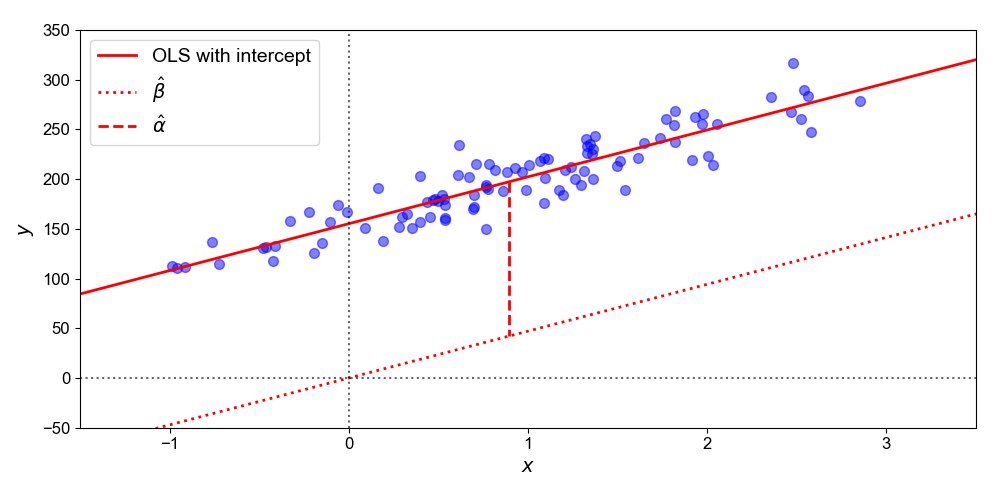
Figure 1. OLS with an intercept (solid line) can be decomposed into OLS without an intercept (dotted line) and intercept term (dashed line). Without an intercept, OLS goes through the origin. With an intercept, the hyperplane is shifted by the distance between the original hyperplane and the mean of the data.

I find it useful to visualize these two parameter estimates (Figure $1$). The slope $\hat{\beta}$ passes through the origin $(0, 0)$, while the intercept $\hat{\alpha}$ shifts this slope so that it passes through the data’s mean, $(\bar{x}, \bar{y})$.

$\hat{\beta}$ in terms of correlation

We can write $\hat{\beta}$ in terms of Pearson’s correlation between our targets $\mathbf{y}$ and predictors $\mathbf{x}$, denoted $\rho_{xy}$. First, let’s denote the sample standard deviations for $\mathbf{x}$ and $\mathbf{y}$ as $S_x$ and $S_y$ respectively, i.e.

$S_x \triangleq \sqrt{\frac{1}{N} \sum_{n=1}^N (x_n - \bar{x})^2}, \qquad S_y \triangleq \sqrt{\frac{1}{N} \sum_{n=1}^N (y_n - \bar{y})^2}. \tag{8}$

Now note that $\hat{\beta}$ in Equation $7$ can be written in terms of the covariance of $\mathbf{x}$ and $\mathbf{y}$ (numerator) and variance of $\mathbf{x}$ (denominator). This is because

$\begin{aligned} \sum_{n=1}^N x_n y_n - \frac{1}{N} \sum_{n=1}^N y_n \sum_{n=1}^N x_n &= \sum_{n=1}^N (x_n - \bar{x})(y_n - \bar{y}) \triangleq N S_{xy}, \\ \sum_{n=1}^N x_n^2 - \frac{1}{N} \sum_{n=1}^N x_n \sum_{n=1}^N x_n &= \sum_{n=1}^N (x_n - \bar{x})^2 \triangleq N S_{x}^2. \end{aligned} \tag{9}$

See A1 for complete derivations of each. Then we can write $\hat{\beta}$ in terms of covariance and variance,

$\hat{\beta} = \frac{\sum_{n=1}^N (x_n - \bar{x})(y_n - \bar{y})}{\sum_{n=1}^N (x_n - \bar{x})^2} = \frac{S_{xy}}{S_{x}^2}, \tag{10}$

which in turn can be written in terms of Pearson’s correlation coefficient $\rho_{xy}$,

$\begin{aligned} \hat{\beta} &= \overbrace{\left( \frac{\sum_{n=1}^N (x_n - \bar{x}) (y_n - \bar{y})}{\sqrt{\sum_{n=1}^N (x_n - \bar{x})^2} \sqrt{\sum_{n=1}^N (y_n - \bar{y})^2}} \right)}^{\rho_{xy}} \left( \frac{\sqrt{\sum_{n=1}^N (y_n - \bar{y})^2}}{\sqrt{\sum_{n=1}^N (x_n - \bar{x})^2}} \right) \\ &= \rho_{xy} \frac{\sqrt{\sum_{n=1}^N (y_n - \bar{y})^2}}{\sqrt{\sum_{n=1}^N (x_n - \bar{x})^2}} \\ &= \rho_{xy} \frac{S_y}{S_x}. \end{aligned} \tag{11}$

In other words, if we standardize our data, the estimated slope $\hat{\beta}$ is just $\rho_{xy}$, the correlation between $\mathbf{x}$ and $\mathbf{y}$. Note that if we were to use OLS without an intercept, we must also mean-center our data for this claim to be true. This is because $\hat{\beta}$ without an intercept is

$\hat{\beta} = \frac{\sum_{n=1}^N x_n y_n}{\sum_{n=1}^N x_n^2}. \tag{12}$

See A2 for a derivation.

Since OLS predicts $\hat{y} = \hat{\alpha} + \hat{\beta} x$, we can write our predictions in terms of the correlation:

$\begin{aligned} \hat{y} &= \hat{\alpha} + \hat{\beta} x \\ \hat{y} &= (\bar{y} - \hat{\beta} \bar{x}) + \hat{\beta} x \\ \hat{y} &= \bar{y} + \hat{\beta}(x - \bar{x}) \\ \hat{y} - \bar{y} &= \left( \rho_{xy} \frac{S_y}{S_x}\right)(x - \bar{x}) \\ &\Downarrow \\ \frac{\hat{y} - \bar{\hat{y}}}{S_y} &= \rho_{xy} \left( \frac{x - \bar{x}}{S_x} \right). \end{aligned} \tag{13}$

We saw in a previous post that $\bar{y} = \bar{\hat{y}}$.

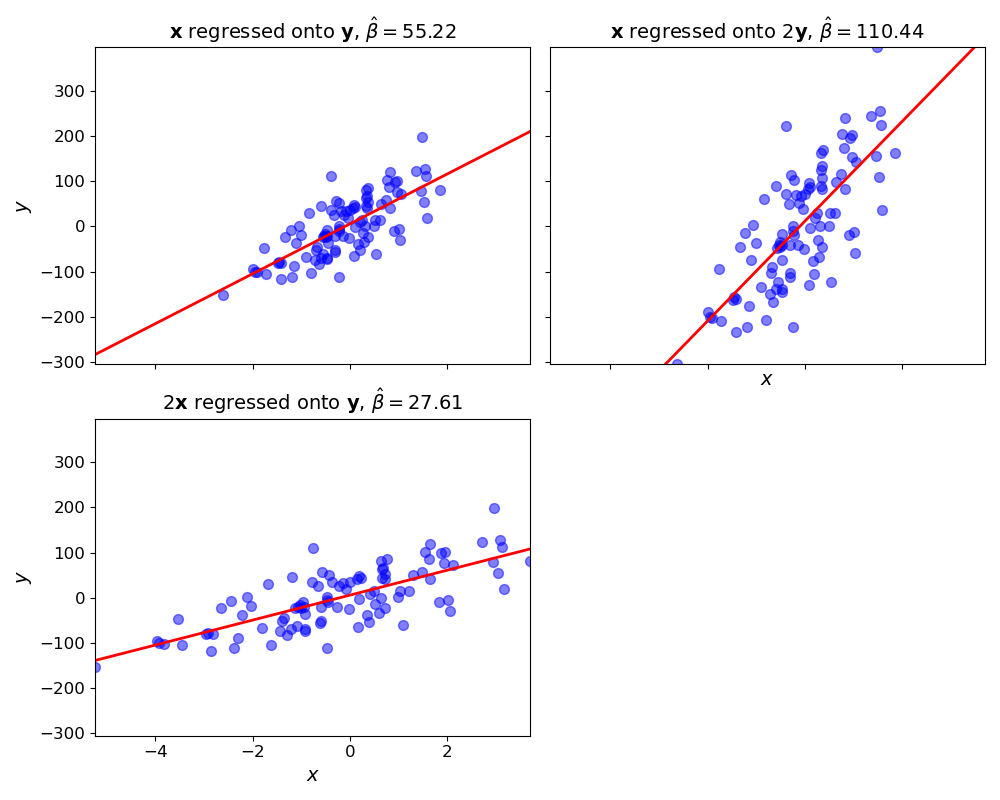
Figure 2. Slope parameter $\hat{\beta}$ for OLS fit to targets and predictors $(\mathbf{x}, \mathbf{y})$ (top left), $(\mathbf{x}, 2 \mathbf{y})$ (top right), and $(2 \mathbf{x}, \mathbf{y})$ (bottom left). The slope halves or doubles, depending on how the standard deviation terms change.

Understanding $\hat{\beta}$ in this way makes it easier to understand implications to changes in our predictors. Example, imagine that we doubled our predictors, i.e. we fit OLS to $2 \mathbf{x} = [2x_1, \dots, 2x_N]^{\top}$ or we doubled our targets, i.e. we fit OLS to $2 \mathbf{y} = [2y_1, \dots, 2y_N]^{\top}$. How would this change our OLS estimates? We know that the correlation would not change, but both the mean and standard deviations would double, so $\hat{\beta}$ would either halve when $\mathbf{x}$ is doubled or double when $\mathbf{y}$ doubles. We can see this directly in Equation $11$, and I have visualized it in Figure $2$.

Acknowledgements

I thank Andrei Margeloiu for pointing out some confusing text regarding when $\hat{\beta}$ is equal to $\rho_{xy}$.

Appendix

A1. Rewriting Equation $7$

Equation $7$’s numerator can be written as the un-normalized sample covariance between $\mathbf{x}$ and $\mathbf{y}$:

$\begin{aligned} &\sum_{n=1}^N x_n y_n - \frac{1}{N} \sum_{n=1}^N y_n \sum_{n=1}^N x_n \\ &= \sum_{n=1}^N x_n y_n - \bar{y} \sum_{n=1}^N x_n - \bar{x} \sum_{n=1}^N y_n + N \frac{1}{N} \sum_{n=1}^N y_n \frac{1}{N} \sum_{n=1}^N x_n \\ &= \sum_{n=1}^N x_n y_n - \bar{y} \sum_{n=1}^N x_n - \bar{x} \sum_{n=1}^N y_n + N \bar{y} \bar{x} \\ &= \sum_{n=1}^N (x_n - \bar{x})(y_n - \bar{y}). \end{aligned} \tag{A1.1}$

Equation $7$’s denominator can be written as the un-normalized sample variance of $\mathbf{x}$:

$\begin{aligned} &\sum_{n=1}^N x_n^2 - \frac{1}{N} \sum_{n=1}^N x_n \sum_{n=1}^N x_n \\ &= \sum_{n=1}^N x_n^2 - 2 \frac{1}{N} \sum_{n=1}^N x_n \sum_{n=1}^N x_n + N \frac{1}{N} \sum_{n=1}^N x_n \frac{1}{N} \sum_{n=1}^N x_n \\ &= \sum_{n=1}^N x_n^2 - 2 \bar{x} \sum_{n=1}^N x_n + N \bar{x}^2 \\ &= \sum_{n=1}^N (x_n - \bar{x}) (x_n - \bar{x}). \end{aligned} \tag{A1.2}$

A2. OLS estimator without an intercept

Without an intercept $\alpha$, the optimal $\beta$ is

$\begin{aligned} \frac{d J}{d \beta} &= \sum_{n=1}^N \frac{d}{d \beta} (y_n - \beta x_n)^2 \\ &= \sum_{n=1}^N 2 (y_n - \beta x_n) (- x_n) \\ &= 2 \left( \sum_{n=1}^N \beta x_n^2 - x_n y_n \right), \\ &\Downarrow \\ 0 &= 2 \left[ \sum_{n=1}^N \beta x_n^2 - x_n y_n \right], \\ &\Downarrow \\ \beta &= \frac{ \sum_{n=1}^N x_n y_n }{ \sum_{n=1}^N x_n^2 } \end{aligned}$

This makes sense. Here, the optimal $\beta$ does not mean center the data, since an intercept is not a modeling assumption.