In ordinary least squares, the coefficient of determination quantifies the variation in the dependent variables that can be explained by the model. However, this interpretation has a few assumptions which are worth understanding. I explore this metric and the assumptions in detail.
Published
09 August 2021
Consider a linear model
y=Xβ+ε,(1)
where y=[y1,…,yN]⊤ are dependent or target variables, X=[x1,…,xN]⊤ is an N×P design matrix of independent or predictor variables, ε=[ε1,…,εN]⊤ are error terms, and β=[β1,…,βP]⊤ are linear coefficients or model parameters. If we estimate β by solving the following quadratic minimization problem,
The goal of this post is to explain a common metric for goodness-of-fit for OLS, called the coefficient of determination or R2. I’ll start by deriving R2 from the fraction of variance unexplained, without stating all my assumptions. Then I’ll state the assumptions and show that they hold for OLS with an intercept but that they are not true in general. I’ll end with a couple discussion points about R2, such as when R2 can be negative and its relationship to Pearson’s correlation coefficient.
Fraction of variance unexplained
A common metric for the goodness-of-fit of a statistical model is the fraction of the variance of the target variables y which cannot be explained by the model’s predictions y^. The fraction of variance unexplained (FVU) is
The numerator is the variance of our residuals, e≜y−y^, and the denominator is the variance of our target variables. Clearly, the 1/N terms cancel, and we can write FVU in vector notation as
FVU=(y−yˉ)⊤(y−yˉ)(y−y^)⊤(y−y^).(4)
If we have perfect predictions, then y^=y, and FVU is zero. In other words, there is no variation in the targets that our model cannot explain. This is a perfect fit. What should our model do if it has no predictive power? The best thing to try is to simply predict the mean of our targets, yˉ=(1/N)∑nyn. In this case, FVU is one. If the model does worse than predicting the mean of the targets, then FVU can be greater than one.
Coefficient of determination
Under certain assumptions, we can derive a new metric from FVU. For now, assume these unspoken assumptions hold. Then the denominator in Equation 4 can be decomposed as
The cancellations are not true in general, and depend on the aforementioned assumptions. But if they hold, then we can write Equation 5 in vector notation in terms of FVU in Equation 4:
The fraction on the left-hand side of Equation 5 is just one minus FVU. This fraction is called the coefficient of determination or R2:
R2=1−FVU.(7)
Thus, R2 is simply one minus the fraction of variance unexplained. When R2 is one, our model has perfect predictive power. This occurs when the residuals e are all zero. When R2 is zero, our model has simply predicted the mean, and y^n=yˉ for all n.
The terms in Equation 6 are important enough to all have names. The numerator in the FVU term is called the residual sum of squares (RSS), since it the squared difference between the true and predicted values, or the residuals. The denominator in the FVU term is called the total sum of squares (TSS), since it is the total variation in our target variables. Finally the numerator on the left-hand-side of Equation 6 is called explained sum of squares (ESS), which is the squared difference between the predictions and mean of our targets. To summarize:
(y−yˉ)⊤(y−yˉ),(y−y^)⊤(y−y^),(y^−yˉ)⊤(y^−yˉ).total sum of squares (TSS)residual sum of squares (RSS)explained sum of squares (ESS)(8)
Using this terminology, Equation 6 says that the total sum of squares decomposes into the explained and residual sum of squares. In other words, the variation in our observations can be explained by OLS in terms of the variation in our residuals and the variation in our regression predictions.
OLS with an intercept
In the previous section, we derived R2 in Equation 5 through two cancellations. When do these cancellations hold? They hold when we assume OLS has an intercept. Let’s see this.
The first cancellation is
2n=1∑Ny^nen=0.(9)
This is true for OLS because of the normal equation:
X⊤Xβ^00=X⊤y=X⊤(y−Xβ^)=X⊤e.(10)
This implies that
y^⊤e=β^⊤X⊤e=0.(11)
Thus, the first term cancels because our statistical model is OLS. If we did not assume OLS or a linear model that minimizes the sum of squared residuals (Equation 2), then we could not necessarily write FVU in terms of R2. This doesn’t mean that the metric R2 would be meaningless, but it would lose its interpretation as the amount of variation in the dependent variables that is explained by our model’s predictions.
The second cancellation is
2yˉn=1∑Nen=0.(12)
This is true if we assume a constant predictor, i.e. when
X=[cX2],(13)
where X2 is our original design matrix and c is an N vector filled with the constant c. If X has a constant predictor, then the last line of Equation 10 can be written as
This immediately implies that the sum of the residuals is zero:
n=1∑Ncen=cn=1∑N(yn−y^n)=0.(15)
To summarize, R2 can only be interpreted in terms of the fraction of variance unexplained if we assume both OLS and OLS with an intercept. Without these assumptions, the decomposition in Equation 5 is no longer valid, and R2 loses this standard interpretation.
Uncentered R2
What if our model does not contain an intercept? The decomposition in Equation 5 is no longer valid. However, the centered total sum of squares still decomposes as
Again, the step labeled ⋆ holds because 0=X⊤e, meaning that we still assume OLS, just not OLS with an intercept. See A1 for an alternative derivation of this decomposition. We can rewrite Equation 16 to rederive the uncenteredR2, which I’ll denote as Ruc2:
Ruc2≜y⊤yy^⊤y^=1−y⊤ye⊤e.(17)
Since y^⊤y^≥0 and e⊤e≥0 and since
Ruc2=y^⊤y^+e⊤ey^⊤y^,(18)
then 0≤Ruc2≤1. As we can see, this measures the goodness-of-fit of OLS. If the residuals are small, then Ruc2 is close to 1. If the residuals are big, then Ruc2 is close 0.
Negative R2
As we have seen, the centered metric Ruc2 cannot be negative. This is simply an algebraic impossibility given Equation 18. However, in practice, one might find that the coefficient of determination or uncentered R2 can be negative. Why does this occur? There are two scenarios. Let’s look at each in turn.
When we use OLS
If our predictors include a constant, then R2 cannot be negative. We know R2 cannot be negative because this would require
However, the OLS estimator β^ is the minimizer of the sum of squared residuals (see Equation 2). If Equation 19 were true, then β^ would no longer the minimizer. Indeed, the smallest value that R2 can be is when the predictions are simply the target mean. It’s easy to see that this occurs when X is un-informative, i.e. when the predictors are constant. See A2 for a proof.
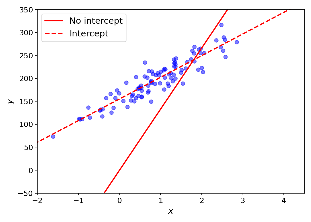
Figure 1. OLS without (red solid line) and with (red dashed line) an intercept. The model's parameters change depending on this modeling assumption.
However, if we do not include an intercept and if our software package still computes R2 using Equation 6, then R2 can be negative. Intuitively, this is because the results of OLS can change dramatically when an intercept is added or removed (Figure 1). In other words, when we do not include an intercept, our model can do much worse than simply predicting the sample mean. Arguably, a negative R2 with OLS is a user error, since it implies the model would do better with the right modeling assumption.
When we do not use OLS
As we saw, the decomposition of the total sum of squares, centered or uncentered, depends on the normal equation, or at least it depends on X⊤e=0. Thus, when using model that is not linear regression, such as a non-linear deep neural network, R2 loses its interpretation as the amount of variation in the target variables that are explained by our predictions, and we have no guarantee that R2 or Ruc2 cannot be negative.
Correlation coefficient squared
The coefficient of determination is called “R2” because it is the square of the Pearson correlation coefficient, which is commonly denoted R, between the targets y and predictions y^. To see this, let’s first write down the correlation coefficient:
Note that we have written yˉ for the mean of the predictions, rather than y^ˉ. This is because yet another important property of OLS with an intercept is that the mean of the predictions equals the mean of the observations, i.e. yˉ=y^ˉ. Why? Since en=yn−y^n by definition, we can write down a relationship between the means of our residuals, predictions, and observations:
Again, this depends on the fact that the residuals sum to zero, as they do when we have a constant predictor in X. Now let’s apply the following simplification to the numerator of Equation 20:
Again, step ⋆ holds since, if we use OLS with an intercept, the residuals sum to zero. See A3 for a complete derivation of this step. Thus, we can write R as
If we square this quantity, we get R2 as in Equation 6.
What this means is that if the targets and predictions are highly negatively or positively correlated, then OLS with an intercept will have a good fit or high R2. As the correlation decreases (regardless of sign), the goodness-of-fit decreases.
Summary
The coefficient of determination is an important metric for quantifying the goodness-of-fit of ordinary least squares. However, its interpretation as the fraction of variance explained by the model depends on the assumption that we are either using OLS with an intercept or we have mean-centered data. A negative R2 is only possible when either not using linear regression or not using linear regression with an intercept. We refer to the coefficient of determination as “R2” because it is the square of Pearson’s correlation coefficient R. When our predictions are either negatively or positively correlated with our regression targets, then a linear model will fit the data better.
The cancellations arise because the matrices are orthogonal to each other, i.e. MH=0.
A2. OLS parameters with un-informative predictors
Consider the scenario in which X is an N×1 matrix of completely un-informative predictors, i.e. a column vector with a constant c. Let’s write this as X≜c=[c,…,c]⊤. Then clearly