The ELBO in Variational Inference

Variational inference

In Bayesian inference, we are often interested in the posterior distribution $p(\mathbf{Z} \mid \mathbf{X})$ where $\mathbf{X}$ are our observations, $\{\mathbf{x}_1, \dots, \mathbf{x}_N\}$ and $\mathbf{Z}$ are latent variables, $\{\mathbf{z}_1, \dots, \mathbf{z}_N\}$. However, in many practical models of interest, this posterior is intractable because we cannot compute the evidence or denominator of Bayes’ theorem, $p(\mathbf{X})$. This evidence is hard to compute because we have introduced latent variables that must now be marginalized out. Such integrals are often intractable in the sense that (1) we do not have an analytic expression for them or (2) they are computationally intractable. See my previous post on HMMs or (Blei et al., 2017) for examples.

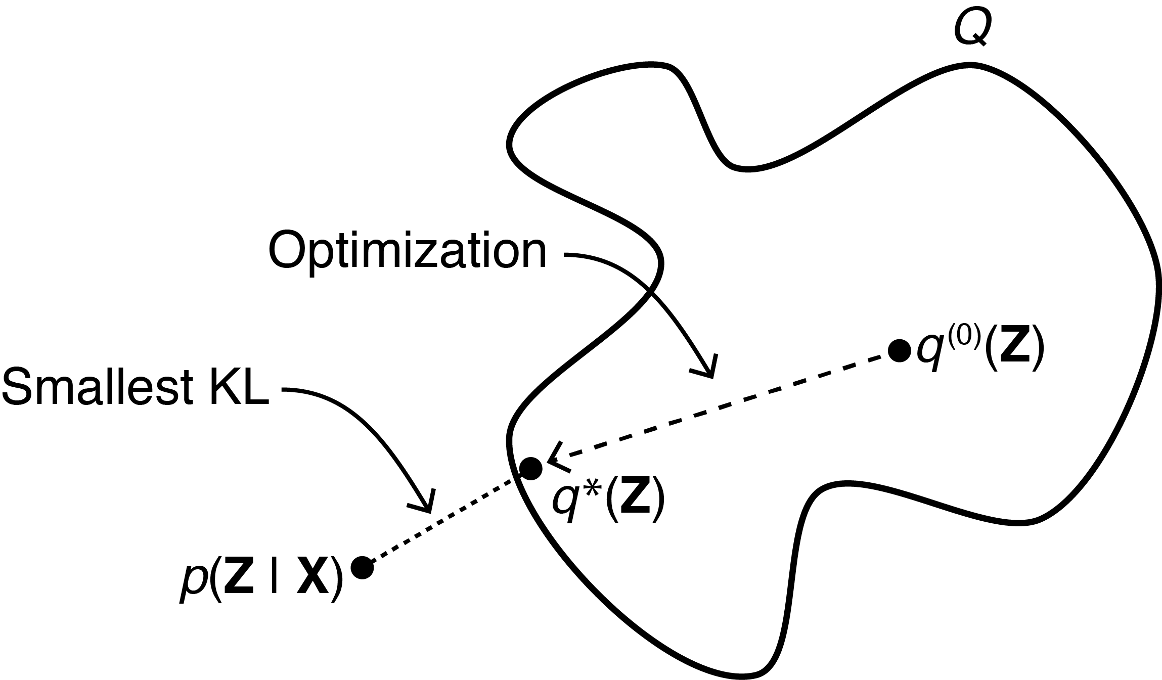
The main idea of variational inference (VI) is to use optimization to find a simpler or more tractable distribution $q(\mathbf{Z})$ from a family of distributions $\mathcal{Q}$ such that it is close to the desired posterior distribution $p(\mathbf{Z} \mid \mathbf{X})$ (Figure $1$). In VI, we define “close to” using the Kullback-Leibler (KL) divergence. Thus, the desired VI objective is

$q^*(\mathbf{Z}) = \arg\!\min_{q(\mathbf{Z}) \in \mathcal{Q}} D_{\text{KL}}[q(\mathbf{Z}) \lVert p(\mathbf{Z} \mid \mathbf{X})]. \tag{1}$

Minimizing the KL divergence can be interpreted as minimizing the relative entropy between the two distributions. See my previous post on the KL divergence for a discussion.

Figure 1. Diagram of VI. A family of distributions $\mathcal{Q}$ is visualized as a blob. VI starts with some initial distribution $q^{(0)}(\mathbf{Z}) \in \mathcal{Q}$ and then iteratively minimizes the KL divergence between the approximating distribution at iteration $t$, call this $q^{(t)}(\mathbf{Z})$, and the desired posterior $p(\mathbf{Z} \mid \mathbf{X})$. The goal is to find an optimal distribution $q^{*}(\mathbf{Z})$ where optimality is defined as having the smallest possible KL divergence between $q^{*}(\mathbf{Z})$ and $p(\mathbf{Z} \mid \mathbf{X})$.

Evidence-lower bound

The main challenge with the variational inference objective in Eq. $1$ is that it implicitly depends on the evidence, $p(\mathbf{X})$. Thus, we have not yet gotten around the intractability discussed above. To see this dependence, let’s write out the definition of the KL divergence:

$\begin{aligned} D_{\text{KL}}[q(\mathbf{Z}) \lVert p(\mathbf{Z} | \mathbf{X})] &= \int_{q} q(\mathbf{Z}) \log \frac{q(\mathbf{Z})}{p(\mathbf{Z} | \mathbf{X})} \\ &= \mathbb{E}_{q(\mathbf{Z})}\left[ \log \frac{q(\mathbf{Z})}{p(\mathbf{Z} | \mathbf{X})} \right] \\ &= \underbrace{\mathbb{E}_{q(\mathbf{Z})}[ \log q(\mathbf{Z})] - \mathbb{E}_{q(\mathbf{Z})}[\log p(\mathbf{Z}, \mathbf{X})]}_{-\text{ELBO}(q)} + \log p(\mathbf{X}). \end{aligned} \tag{2}$

Because we cannot compute the desired KL divergence, we optimize a different objective that is equivalent to this KL divergence up to constant. This new objective is called the evidence lower bound or ELBO:

$\text{ELBO}(q) := \mathbb{E}_{q(\mathbf{Z})}[\log p(\mathbf{Z}, \mathbf{X})] - \mathbb{E}_{q(\mathbf{Z})}[ \log q(\mathbf{Z})]. \tag{3}$

This is a negation of the left two terms in Eq. $2$. We can rewrite Eq. $2$ as

$\log p(\mathbf{X}) = \text{ELBO}(q) + D_{\text{KL}}[q(\mathbf{Z}) \lVert p(\mathbf{Z} | \mathbf{X})]. \tag{4}$

Why is the ELBO so-named? Since the KL divergence is non-negative, we know

$\log p(\mathbf{X}) \geq \text{ELBO}(q). \tag{5}$

In other words, the log evidence $\log p(\mathbf{X})$, a fixed quantity for any set of observations $\mathbf{X}$, cannot be less than the ELBO. So if we maximize the ELBO, we minimize the desired KL divergence. This is VI in a nutshell.

Relationship to EM

It’s fun to observe the relationship between VI and expectation–maximization (EM). EM maximizes the expected log likelihood when $q(\mathbf{Z}) = p(\mathbf{Z} | \mathbf{X})$, i.e.

$\log p(\mathbf{X}) = \overbrace{\vphantom{\Big|}\text{ELBO}(q)}^{\text{EM maximizes this}} + \overbrace{\vphantom{\Big|} \text{KL}[q(\mathbf{Z}) \lVert p(\mathbf{Z} | \mathbf{X})]}^{\text{Since this is zero}}. \tag{6}$

To be a bit more pedantic, at iteration $t$ with current parameters estimates $\boldsymbol{\theta}^{(t)}$, EM optimizes this expected complete log likelihood inside the ELBO:

$\log p(\mathbf{X} \mid \boldsymbol{\theta}) = \overbrace{\mathbb{E}_{p(\mathbf{Z} \mid \mathbf{X}, \boldsymbol{\theta}^{(t)})} \left[ \log p(\mathbf{X}, \mathbf{Z} \mid \boldsymbol{\theta})\right]}^{\text{EM maximizes this}} - \mathbb{E}_{p(\mathbf{Z} \mid \mathbf{X}, \boldsymbol{\theta}^{(t)})} \left[ \log p(\mathbf{Z} \mid \mathbf{X}) \right]. \tag{7}$

See my previous post on EM for why EM ignores the right term in Eq. $7$.

Gradient-based VI

VI is a framework, and there are a variety of different ways to optimize this ELBO. (See (Blei et al., 2017) for a much deeper discussion.) A popular approach in deep generative modeling is to use gradient-based optimization of the ELBO. Describing a low-variance, gradient-based estimator of the ELBO is a main contribution of (Kingma & Welling, 2013). This allows for us to approximate the posterior with more flexible density estimators, such as neural networks. The most famous example of gradient-based VI is probably the variational autoencoder. See (Kingma & Welling, 2013) or my previous post on the reparameterization trick for details.