Inference for Hidden Markov Models

The simplest probabilistic model of sequential data is that the data are i.i.d. We assume the data are Gaussian or binomial or from a nonparametric distribution we cannot write down, but we do not assume that model changes over time. We do not assume we can make any inference about the next observation given the current one. The graphical model for this assumption would be a sequence of unconnected nodes.

Of course, this assumption prevents modeling any sequential structure. For example, in text, certain words are more likely to follow a given word than others, while an i.i.d. assumption would obliterate this structure by assuming each word is independent from the words around it. One simple model, called a first-order Markov model, is that each observation only depends on the previous one. For example, if we assume that each observation is Gaussian and its mean linearly depends on the previous data point, then we are working with an autoregressive model.

First-order models can be extended to $M$-th order Markov models which assume each observation depends on the previous $M$ observations. However, the number of parameters of this model is exponential in $M$. For example, imagine we flipped a coin $M$ times, and we need to consider all possible sequence of coin flips. Each time $M$ increases by one, the number of possible sequences doubles. Thus, inference is intractable for even modest values of $M$.

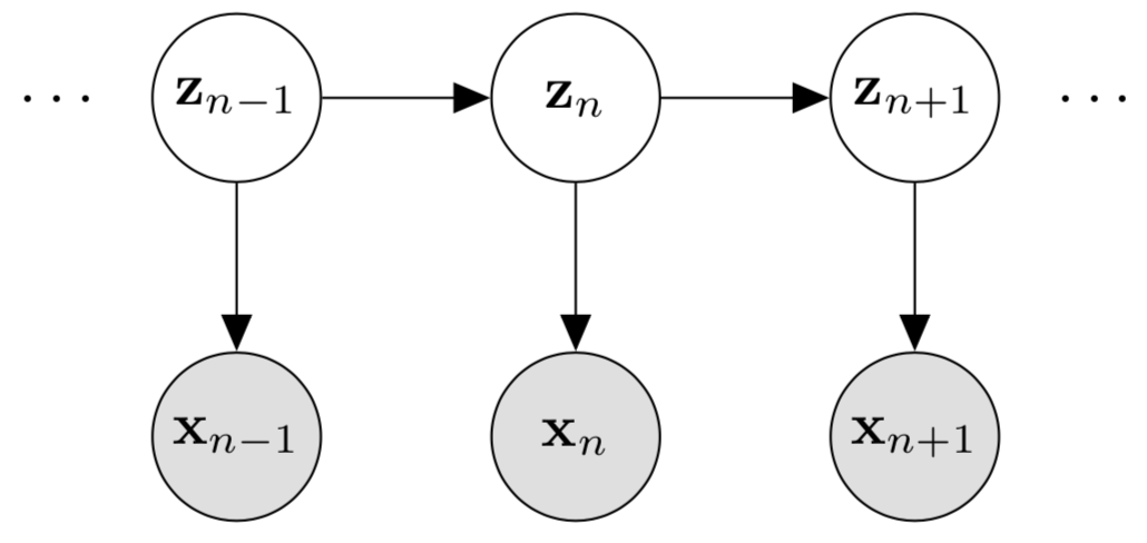
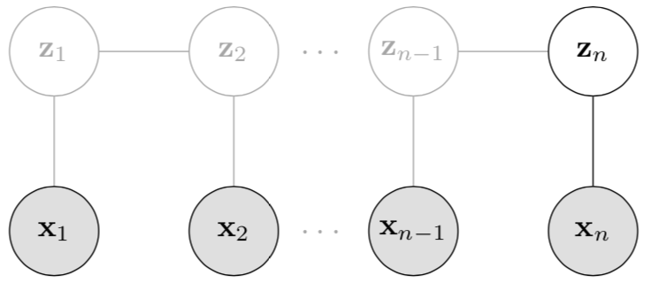
A powerful probabilistic model of sequential data that still limits the number of parameters is the hidden Markov model (HMM). The key idea is that a latent variable or state variable, rather than the data, evolves according to a discrete, first-order Markov process. Each observation is conditionally independent of every other observation given the value of its associated latent variable (Fig. $1$).

Figure 1: Graphical model for a hidden Markov model. The hidden state variables $\mathbf{z}_1, \dots, \mathbf{z}_N$ follow a Markov process, while each observation $\mathbf{x}_n$ is conditionally independent from other data given its associated hidden state variable $\mathbf{z}_n$.

However, and this is the clever bit, notice that no observation is $d$-separated from any other observation. There is always an unblocked path between any two observations because all observations are connected via the latent variables. Thus, our predictive distribution is

$p(\mathbf{x}_{n+1} \mid \mathbf{x}_1, \dots, \mathbf{x}_n), \tag{1}$

meaning that $\mathbf{x}_{n+1}$ depends on all previous observations. Thus, by introducing these latent variables, we can tractably compute a flexible predictive distribution.

The goal of this post is to work through HMMs in detail. In particular, I want to focus on the Baum–Welch and forward–backward algorithms. I assume the reader understands Markov chains and expectation–maximization.

Example: Rainier weather data

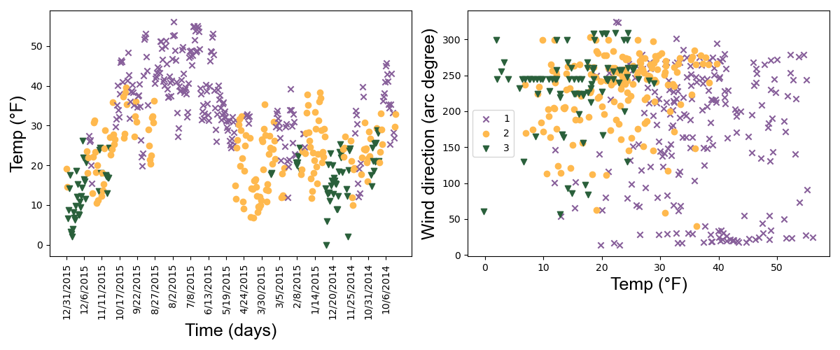
Before diving into the model and inference details, let’s look at an example. I fit a hidden Markov model using the code below on Mount Rainier weather data. The data features are: temperature, relative humidity, daily wind speed, wind direction, and battery voltage. Each feature was collected daily between 3 August 2014 and 31 December 2015. I used three state variables, meaning the HMM will assign each day to one of three latent or hidden states. In Fig. $2$, I plotted temperature across time (left panel) and temperature vs. wind direction (right panel). I colored the data points by their hidden states. As we can see, the inferred states are fairly interpretable, roughly capturing warm, cool, and cold days. Interestingly, it looks like the coldest days on Rainier have wind coming from the south.

Figure 2: Mount Rainier weather data between 3 August 2014 and 31 December 2015 with days. In both plots, days (data points) are labeled by a three-state hidden Markov model. (Left) Temperature across time. (Right) Temperature vs. wind direction.

Probabilistic model

Now that we have an intuition for what kinds of problems HMMs address, let’s dive into the details. Let $\mathbf{X} = \{\mathbf{x}_1, \dots, \mathbf{x}_N\}$ be $N$ sequential observations where $\mathbf{x}_n \in \mathbb{R}^{D}$ where $D$ is a counting number. HMMs assume that each observation $\mathbf{x}_n$ has a corresponding latent variable $\mathbf{z}_n$. We denote this set of latent variables as $\mathbf{Z} = \{\mathbf{z}_1, \dots, \mathbf{z}_N\}$. Note that each $\mathbf{z}_n$ is a one-hot vector, not a scalar. This means $\mathbf{z}_n$ is a $K$-vector—meaning the HMM has $K$ states—with $K-1$ zeros and $1$ one, indicating the assignment. We do this so that we can treat $\mathbf{z}_n$ as a multinomial random variable, e.g.:

$\mathbf{z}_{n} = \begin{bmatrix} 0 \\ 0 \\ 1 \\ 0 \\ \vdots \\ 0 \end{bmatrix}, \tag{2}$

would indicate that the $n$-th latent state is $3$ (using one-based indexing). Why do we use this representation? This lets us think of $\mathbf{z}_n$ as a single draw from a multinomial distribution with parameters $1$ and $[p_1, \dots, p_K]^{\top}$.

Markov assumption

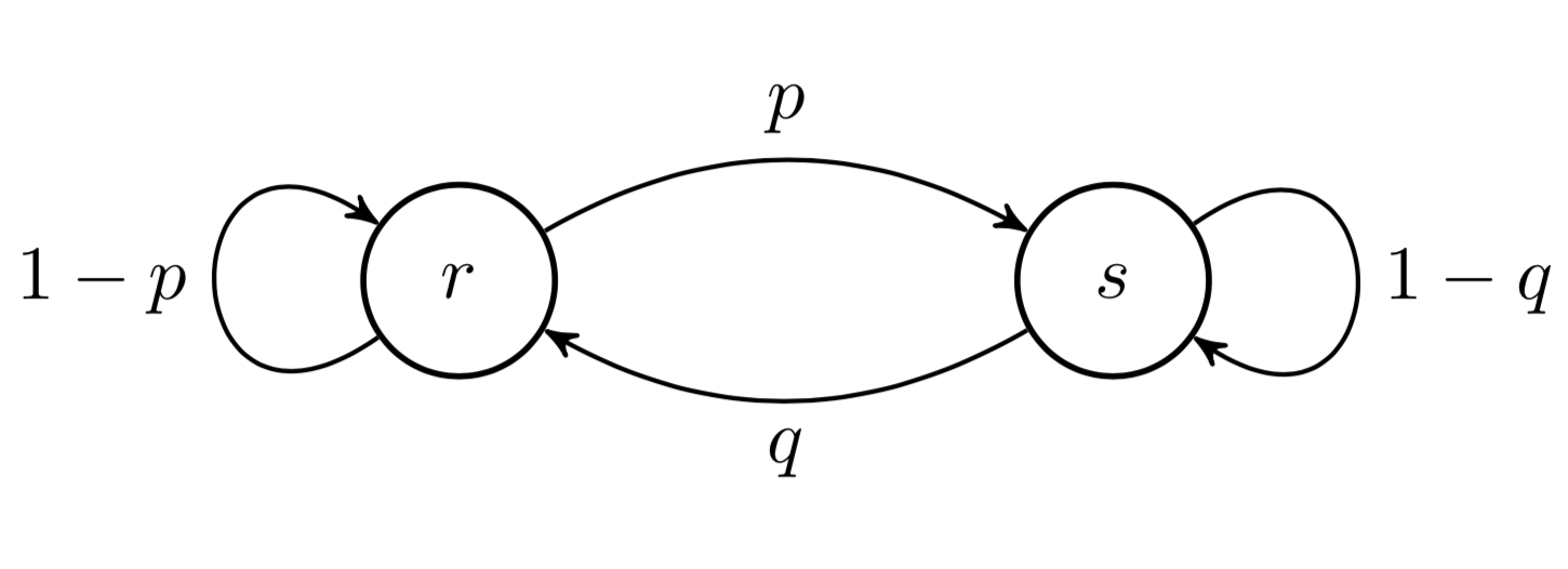
We assume the latent variables follow a random process, a $K$-state Markov chain. For example, consider a $K = 2$ state Markov chain modeling the weather. The weather can either be sunny ($\mathbf{z}_n = s$) or rainy ($\mathbf{z}_n = r$) at time index $n$ (day, hour, minute, etc.). The transition probabilities are given in Fig. $3$.

Figure 3: State diagram for a Markov chain $\{\mathbf{z}_n\}$ with states $\mathcal{S} = \{r, s\}$. The probability of moving from $r$ to $s$ is $p$ and from $s$ to $r$ is $q$. The remaining probabilities can be computed because probabilities over all disjoint events must sum to one.

For an HMM, imagine that we only observe humidity as a percentage. Thus, at each time point $n$, $\mathbf{x}_n$ is a scalar in the range $[0, 1]$, representings the day’s humidity, while the latent variable $\mathbf{z}_n$ evolves according to the chain in Fig. $3$. Thus, if we could infer $\mathbf{Z}$, we could cluster our humidity data into $K=2$ states.

The random process $\mathbf{Z}$ is first-order Markovian. This Markov assumption is that the future only depends on the present. Formally, a random process $\mathbf{z}_1, \mathbf{z}_2, \dots$ taking values in $\mathcal{S}$ is called a Markov chain if

$p(\mathbf{z}_{n+1} \mid \mathbf{z}_{n}, \dots, \mathbf{z}_1) = p(\mathbf{z}_{n+1} \mid \mathbf{z}_{n}). \tag{3}$

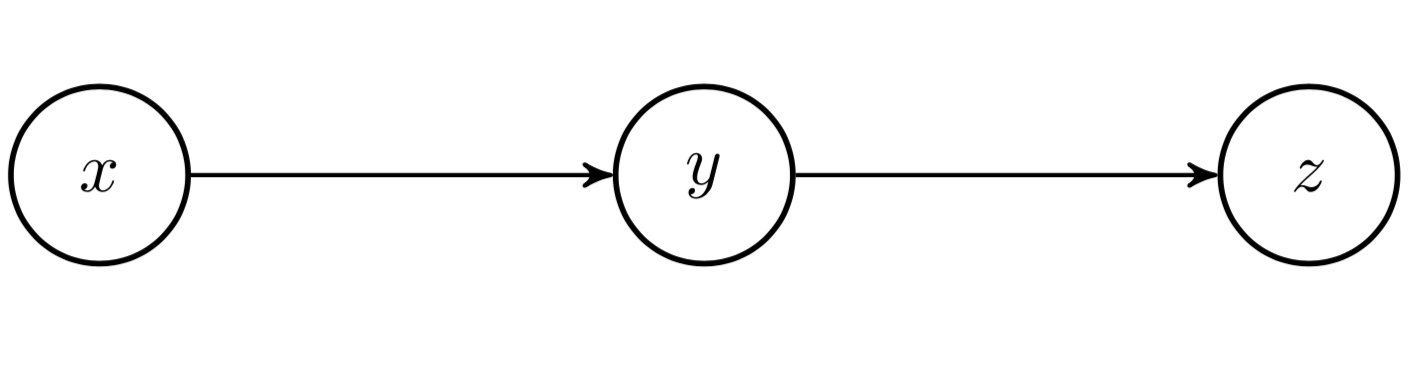
Thus, for a Markov chain such as in Fig. $4$, we can say that $X \perp\!\!\!\!\perp Z \mid Y$, which is read: “$X$ is independent of $Z$ given $Y$”. For example, height and vocabulary are not independent. In the absence of any other information, we might guess that someone who is six-feet tall has a bigger vocabulary than someone who is four-feet tall. However, height and vocabulary are conditionally independent given age. If we learn that the six-foot tall person is a fast-growing fourteen-year-old while the the four-foot tall person is thirty-five, we might switch our guess as to who has the bigger vocabulary. In Fig. $4$, “vocabulary” is the $Z$ node, height is the $Y$ node, and age is the $X$ node. We can see that if we don’t know $Y$, we can use $X$ to infer $Z$; but if we do know $Y$, $X$ is irrelevant.

Figure 4: Graphical model in which state $Z$ is conditionally independent from $X$ given $Z$.

An important implication of the Markovian assumption is that the joint probability of our HMM factorizes nicely,

$\begin{aligned} p(\mathbf{Z}) &= p(\mathbf{z}_1) p(\mathbf{z}_2 \mid \mathbf{z}_1) p(\mathbf{z}_3 \mid \mathbf{z}_2, \mathbf{z}_1) \dots p(\mathbf{z}_N \mid \mathbf{z}_{N-1}, \dots, \mathbf{z}_1) \\ &= p(\mathbf{z}_1) p(\mathbf{z}_2 \mid \mathbf{z}_1) p(\mathbf{z}_3 \mid \mathbf{z}_2) \dots p(\mathbf{z}_N \mid \mathbf{z}_{N-1}) \\ &= p(\mathbf{z}_1) \prod_{n=1}^{N} p(\mathbf{z}_{n+1} \mid \mathbf{z}_n). \end{aligned} \tag{4}$

Because of this factorization, the joint probability $p(\mathbf{Z})$ can be completely represented via a transition probability matrix. Let $A_{ij}$ be the probability of transitioning from state $i$ to state $j$. Then the transition probability matrix is $\mathbf{A} = [A_{ij}]_{i,j \in S}$. Since there are $K$ states, $\mathbf{A}$ is a $K \times K$ matrix. Furthermore, we assume the Markov process is stationary or time-homogeneous, meaning

$p(\mathbf{z}_n = j \mid \mathbf{z}_n = i) = A_{ij}, \quad \forall n. \tag{5}$

In words, the transition probabilities are not changing as a function of $n$. This assumption can be changed to produce a time-inhomogeneous Markov chain, but we’ll focus on the time-homogeneous model.

Emission probabilities

In addition to the transition probabilities, an HMM has emission probabilities, which model how we assume our data are distributed given the state variable $\mathbf{z}_n$:

$p(\mathbf{x}_n \mid \mathbf{z}_n = k, \boldsymbol{\phi}_k), \tag{6}$

where $\boldsymbol{\phi}_k$ are the parameters of some distribution which we posit. For example, we might model $\mathbf{x}_n$ as a $D$-variate normal given $\mathbf{z}_n$ or

$\mathbf{x}_n \sim \mathcal{N}_D(\mathbf{x}_n \mid \boldsymbol{\mu}_k, \boldsymbol{\Sigma}_k). \tag{7}$

Thus, $\mathbf{z}_n$ indexes the parameter of the distribution, meaning it specifies which parameters to use in the set $\{\boldsymbol{\phi}_k\}_{k=1}^{K}$ at time $n$. Clearly, these probabilities are of interest because if we infer $\mathbf{z}_n$, then the emission probabilities tell us something about our data. For example, in the Mount Rainier example, I fit a Gaussian HMM; the Gaussian mean vector $\boldsymbol{\mu}_k$ for each of the three states tells us the mean value for the data vector $\mathbf{x}_n$.

Initialization

The last thing to note is how to initialize the state distribution of our Markov chain. Let $\boldsymbol{\pi}$ be a $K$-dimensional vector representing the probability of the Markov chain starting on each of the $K$ states. Thus, the components of $\boldsymbol{\pi}$ sum to one, $\sum_{k=1}^{K} \pi_k = 1$, and $\boldsymbol{\pi}$ is called the initial state distribution. Recall that a multinomial random variable with parameters $(M, \pi_1, \dots, \pi_K)$ models the probability of rolling a $K$-sided die $M$ times, where $\pi_k$ is the bias of the die landing on the $k$th side. With $M = 1$ and $\boldsymbol{\pi} = [ \pi_1, \dots, \pi_K ]^{\top}$, we can express our modeling assumption about $\mathbf{z}_1$ taking one of $K$ values as a multinomial random variable,

$\mathbf{z}_1 \sim \text{Mult}(1, \boldsymbol{\pi}). \tag{8}$

HMMs can be either supervised or unsupervised. In the supervised setting, our observations have state labels $\mathbf{X} = \{(\mathbf{x}_1, \mathbf{z}_1), \dots, (\mathbf{x}_N, \mathbf{z}_N)\}$. In this context, we can use empirical Bayes to estimate $\boldsymbol{\pi}$,

$\hat{\pi}_k = \frac{\sum_{n=1}^{N} \mathbf{1}(\mathbf{z}_n = k)}{N} \tag{9}$

where $\mathbf{1}(\mathbf{z}_n = k)$ is an indicator random variable. The goal of a supervised HMM is to estimate the initial state, the transition probability matrix $\mathbf{A}$, and the emission probabilities $p(\mathbf{x}_n \mid \mathbf{z}_n, \boldsymbol{\phi})$. This post will focus on the unsupervised setting. In this case, we need to estimate the model parameters $\boldsymbol{\theta} = \{\boldsymbol{\pi}, \mathbf{A}, \boldsymbol{\phi} \}$ (the initial state, the transition probability matrix, and the emission probabilities) and the state variables $\mathbf{Z}$.

Filtering and smoothing

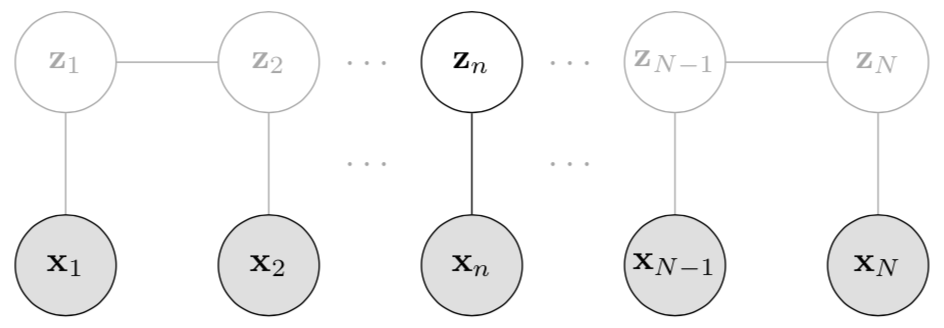
Before discussing inference, it is helpful to discuss two concepts in the HMM literature: filtering and smoothing. Filtering computes a belief state, or the probability of the latent variable $\mathbf{z}_n$ being on a certain state in $\mathcal{S}$, given the history of evidence so far (Fig. $5$). Formally, filtering computes

$p(\mathbf{z}_n \mid \mathbf{X}_{1:n}), \tag{10}$

where the notation $\mathbf{X}_{a:b}$ denotes the set $\{ \mathbf{x}_a, \mathbf{x}_{a+1}, \dots, \mathbf{x}_{b-1}, \mathbf{x}_b \}$ for $a \leq b$. Using our running example of weather, filtering answers the question: given weather measurements up until the current time, what state are we in now? Notice that the Markov property forces us to look at all of our observations. This is because of how the model factorizes. Since the dependencies between time points are encoded in the random process, we need to marginalize over all of the previous latent variables to condition on $\mathbf{X}_{1:n}$.

Figure 5: Filtering or posterior inference of $\mathbf{z}_n$ given all the observations up until that time point, $\mathbf{x}_1, \dots, \mathbf{x}_n$.

As we’ll see, the forward–backward algorithm for HMMs performs filtering in a recursive forward pass over the data. At each time point, it computes it’s belief about the current $\mathbf{z}_n$ and then uses that estimate in its estimate for $\mathbf{z}_{n+1}$.

In smoothing, we compute a belief state given observations up to and including future time, relative to $\mathbf{z}_n$ (Fig. $6$). Formally,

$p(\mathbf{z}_n \mid \mathbf{X}). \tag{11}$

For example, smoothing answers the question: given all the weather measurement data available to us, what state were we in some time period ago? Once again, since the dependencies between time points are encoded in the random process, to condition on $\mathbf{x}_{1:N}$ requires marginalizing over all the latent variables. Thus, we cannot look at fewer than all our observations.

Figure 6: Smoothing or posterior inference of $\mathbf{z}_n$ given all the observations $\mathbf{x}_1, \dots, \mathbf{x}_N$.

Smoothing is performed during the backward pass of the forward–backward algorithm. You can think of it as “smoothing” because we’re using all the data we have seen so far to update our original, filtering-based estimate of each $\mathbf{z}_n$.

There are a number of other tasks we can perform with HMMs. Prediction computes $p(\mathbf{x}_{n+1} \mid \mathbf{x}_{1:n})$. Viterbi decoding labels the most likely states for a new observed sequence $\mathbf{x}_{1:M}$. Posterior sampling allows us to randomly sample a latent state sequence $\mathbf{z}_{1:N}$ given an observed sequence $\mathbf{x}_{1:N}$. In this post, we’ll focus on just filtering and smoothing, since these two steps are the core components of the forward–backward algorithm for HMM inference.

Baum–Welch algorithm

To perform maximum likelihood estimation on an HMM, we need to compute the likelihood $p(\mathbf{X} \mid \boldsymbol{\theta})$ for $\boldsymbol{\theta} = \{\boldsymbol{\pi}, \mathbf{A}, \boldsymbol{\phi}\}$. We could compute this by marginalizing over the latent variables,

$p(\mathbf{X} \mid \boldsymbol{\theta}) = \sum_{\mathbf{Z}} p(\mathbf{X}, \mathbf{Z} \mid \boldsymbol{\theta}). \tag{12}$

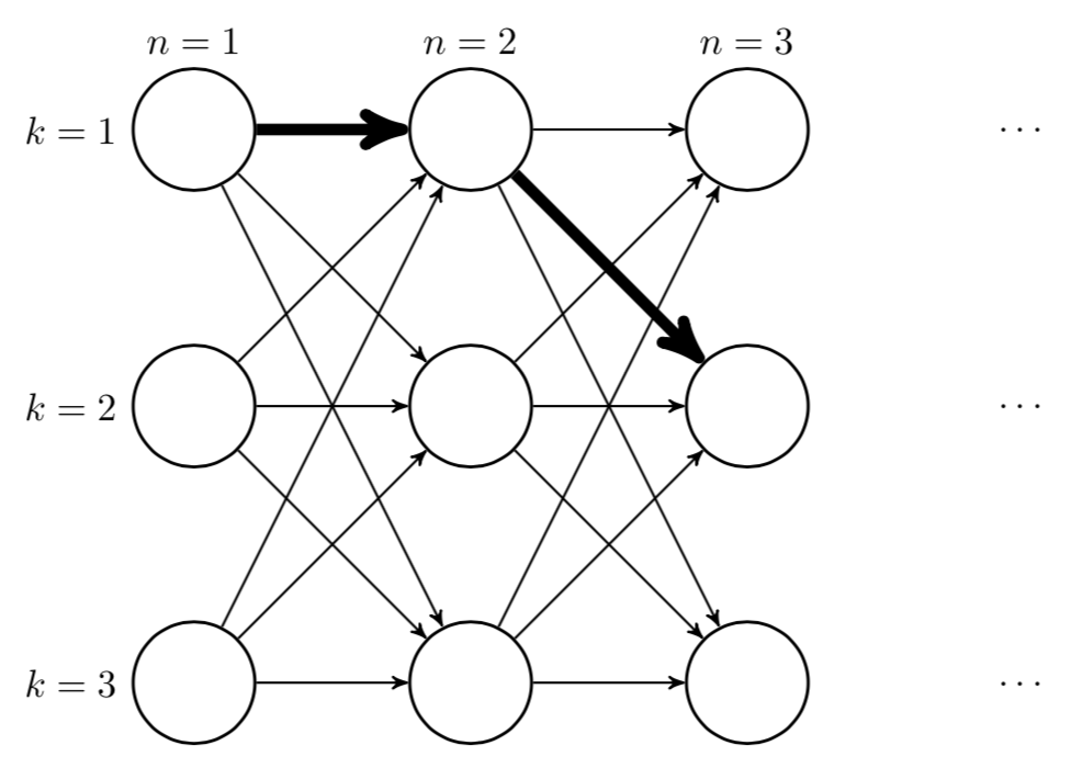
In words, we could marginalize out our uncertainty of the state variables by considering all possible values. However, there are $K^N$ terms in this equation. This is because for all $N$ observations, there are $K$ possible state values at time $n$. To see this, consider Fig. $7$. Here we unroll an HMM with $K=3$ states, representing all possible state values over time. A single configuration of $\mathbf{Z}$—a single term in the sum in Eq. $12$—amounts to a single path along the lattice in Fig. $7$. There are $K^N$ such paths. Since the number of terms in the likelihood scales exponentially in $N$, computing $p(\mathbf{X} \mid \boldsymbol{\theta})$ directly is intractable.

Figure 7: Unrolling a $K=3$ state HMM into a $K \times N$ lattice. The bolded path is a single set of assignments $\mathbf{Z}$.

The standard solution to this kind of problem is expectation–maximization (EM). As we’ll see, the inference algorithm is a bit more complicated than “just EM”, and it has a name, the Baum–Welch algorithm (Baum et al., 1970). The M-step of the Baum–Welch algorithm is fairly straightforward, but the E-step is tricky and leverages the forward–backward algorithm.

EM works by iteratively optimizing the expected complete log likelihood rather than $\log p(\mathbf{X} \mid \boldsymbol{\theta})$. It consists of two eponymous steps:

$\begin{aligned} \textbf{E-step:} && Q(\boldsymbol{\theta} \mid \boldsymbol{\theta}^{(t)}) &= \mathbb{E}_{p(\mathbf{Z} \mid \mathbf{X}, \boldsymbol{\theta}^{(t)})} \big[ \log p(\mathbf{X}, \mathbf{Z} \mid \boldsymbol{\theta})\big] \\ \textbf{M-step:} && \boldsymbol{\theta}^{(t+1)} &= \arg\!\max_{\boldsymbol{\theta}} Q(\boldsymbol{\theta} \mid \boldsymbol{\theta}^{(t)}). \end{aligned} \tag{13}$

In the E-step, we construct a tight lower bound to the log likelihood. In the M-step, we optimize this lower bound. EM relies on the fact that it is often easier to optimize the complete log likelihood $p(\mathbf{X}, \mathbf{Z} \mid \boldsymbol{\theta})$ than it is to optimize the log likelihood $p(\mathbf{X} \mid \boldsymbol{\theta})$. We also want to estimate the parameters $\boldsymbol{\theta}$ under the modeling assumption that $\mathbf{Z}$ exists, and therefore we need the M-step. In more detail, our two steps are:

$\begin{aligned} \textbf{E-step:} &&& \text{Estimate $\mathbb{E}[\mathbf{Z}^{(t+1)} \mid \mathbf{X}, \boldsymbol{\theta}]$ given $\mathbf{X}$, $\boldsymbol{\pi}^{(t)}, \mathbf{A}^{(t)}$ and $\boldsymbol{\phi}^{(t)}$.} \\ \textbf{M-step:} &&& \text{Estimate $\boldsymbol{\pi}^{(t+1)}, \mathbf{A}^{(t+1)}$ and $\boldsymbol{\phi}^{(t+1)}$ given $\mathbb{E}[\mathbf{Z}^{(t+1)} \mid \mathbf{X}, \boldsymbol{\theta}]$ and $\mathbf{X}$.} \end{aligned} \tag{14}$

We use the expectations in Eq. $14$ to compute the expected complete log likelihood. As we will see, we compute the E-step using the forward–backward algorithm; and we compute the M-step using maximum likelihood estimation and Lagrange multipliers.

E-step

First, let’s construct the complete log likelihood:

$\begin{aligned} \log p(\mathbf{Z}, \mathbf{X} \mid \boldsymbol{\theta}) &= \log \Big\{ p(\mathbf{z}_1) \Big[ \prod_{n=2}^{N} p(\mathbf{z}_{n} \mid \mathbf{z}_{n-1}) \Big] \Big[ \prod_{n=1}^{N} p(\mathbf{x}_n \mid \mathbf{z}_n) \Big] \Big\} \\ &= \log p(\mathbf{z}_1) + \sum_{n=2}^{N} \log p(\mathbf{z}_{n} \mid \mathbf{z}_{n-1}) + \sum_{n=1}^{N} \log p(\mathbf{x}_n \mid \mathbf{z}_n). \end{aligned} \tag{15}$

Let $\boldsymbol{\theta}^{(t)}$ denote the current parameter estimates. We’ll estimate $\boldsymbol{\theta}^{(t+1)}$ in the M-step. The expected complete log likelihood is

$\begin{aligned} &\mathbb{E}_{p(\mathbf{Z} \mid \textbf{X}, \boldsymbol{\theta}^{(t)})} \big[\log p(\mathbf{Z}, \mathbf{X} \mid \boldsymbol{\theta}^{(t)})\big] \\ &= \mathbb{E} \big[\log p(\mathbf{z}_1)\big] + \mathbb{E} \big[ \sum_{n=2}^{N} \log p(\mathbf{z}_{n} \mid \mathbf{z}_{n-1})\big] + \mathbb{E} \big[ \sum_{n=1}^{N} \log p(\mathbf{x}_n \mid \mathbf{z}_n)\big]. \end{aligned} \tag{16}$

Now recall that we’re conditioning on our parameter estimates $\boldsymbol{\theta}^{(t)} = \{\boldsymbol{\pi}^{(t)}, \mathbf{A}^{(t)}, \boldsymbol{\phi}^{(t)}\}$, and the only randomness is in the latent state variables $\mathbf{Z}$, which is a collection of multinomial random variables. So let’s write each expectation as explicit sums over the state variables:

$\sum_{k=1}^{K} \mathbb{E}[ z_{1k} ] \log \pi_k + \sum_{n=2}^{N} \sum_{j=1}^K \sum_{k=1}^K \mathbb{E}[z_{n-1,j} z_{nk}] \log A_{jk} + \sum_{n=1}^{N} \sum_{k=1}^{K} \mathbb{E}[z_{nk}] \log p(\mathbf{x}_n \mid \boldsymbol{\phi}_k). \tag{17}$

Here, $z_{nk}$ is the $k$-th component of the vector $\mathbf{z}_n$. See A1 for a complete derivation of Eq. $17$. This might seem like a turgid representation, but it has two benefits. First, we have isolated the random quantities; and second, we have written everything explicitly in terms of our parameters $\boldsymbol{\theta}$. Since the E-step amounts to estimating $\mathbf{Z}$ under the expected complete log likelihood, we just need to compute the terms inside expectations in Eq. $17$ given our parameters $\boldsymbol{\theta}$ and then use those expectations in the M-step. We don’t actually have to compute the value of the expected complete log likelihood.

Now note that each $z_{nk}$ is a component of a multinomial random variable $\mathbf{z}_n$. So the expectation is just the probability that $z_{nk}$ takes the value $1$:

$\begin{aligned} \mathbb{E}[z_{nk}] &= \sum_{k^{\prime}=1}^{K} z_{nk} p(\mathbf{z} = k^{\prime} \mid \mathbf{X}, \boldsymbol{\theta}^{(t)}), \\ \mathbb{E}[z_{n-1, j} z_{nk}] &= \sum_{k^{\prime}=1}^{K} z_{n-1,j} z_{nk} p(\mathbf{z} = k^{\prime} \mid \mathbf{X}, \boldsymbol{\theta}^{(t)}). \end{aligned} \tag{18}$

In the sum, $K-1$ terms are $0$ because $\mathbf{z}$ is a one-hot vector.

The goal of the E-step is to efficiently compute these posterior moments (Eq. $18$), and this is done using the forward–backward algorithm. Following Bishop, I will refer to the these posterior moments as gamma ($\gamma$) and xi ($\xi$) respectively:

$\begin{aligned} \gamma(z_{nk}) &= \mathbb{E}[z_{nk}], \\ \xi(z_{n-1,j}, z_{nk}) &= \mathbb{E}[z_{n-1, j} z_{nk}]. \end{aligned} \tag{19}$

The forward–backward algorithm estimates $\gamma(z_{nk})$ and $\xi(z_{n-1,j}, z_{nk})$ for every $n \in \{1, \dots, N\}$ and every $k \in \{1, \dots, K\}$. We’ll walk through the algorithm in detail in the next section, but now let’s look at the M-step.

M-step

In the M-step, we want to maximize the parameters, $\boldsymbol{\theta} = \{\boldsymbol{\pi}, \mathbf{A}, \boldsymbol{\phi}\}$, given $\mathbf{Z}^{(t)}$. The first two parameters can be optimized using Lagrange multipliers. Let’s walk through optimizing $\boldsymbol{\pi}$ in detail. The Lagrangian function for $\boldsymbol{\pi}$ is

$L(\boldsymbol{\pi}, \lambda_{\pi}) = \underbrace{\sum_{k=1}^{K} \mathbb{E}[z_{1k}] \log \pi_k + \dots}_{Q(\boldsymbol{\theta} \mid \boldsymbol{\theta}^{(t)})} + \lambda_{\pi} \Big( \sum_{k=1}^K \pi_k - 1 \Big), \tag{20}$

where $\lambda_{\pi}$ is the Lagrange multiplier for $\boldsymbol{\pi}$ and where “$\dots$” represent the other terms in Eq. $17$ that do not depend on $\boldsymbol{\pi}$. The partial derivatives of this function with respect to both each $\pi_k$ and $\lambda_{\pi}$ is:

$\begin{aligned} \frac{\partial L(\boldsymbol{\pi}, \lambda_{\pi})}{\partial \pi_k} &= \frac{\mathbb{E}[z_{1k}]}{\pi_k} + \lambda_{\pi}, \\ \frac{\partial L(\boldsymbol{\pi}, \lambda_{\pi})}{\partial \lambda_{\pi}} &= \sum_{k=1}^{K} \pi_k - 1. \end{aligned} \tag{21}$

We set these equal to zero and solve the system of equations. We can write each $\pi_k$ in terms of $\lambda_{\pi}$:

$\frac{\mathbb{E}[z_{1k}]}{\pi_k} + \lambda_{\pi} = 0 \iff \pi_k = - \frac{\mathbb{E}[z_{1k}]}{\lambda_{\pi}}. \tag{22}$

We can plug this into the second equation in Eq. $21$ to solve for $\lambda_{\pi}$:

$\sum_{k=1}^{K} \pi_k - 1 = 0 \iff \sum_{k=1}^{K} \Big( - \frac{\mathbb{E}[z_{1k}]}{\lambda_{\pi}} \Big) = 1 \iff -\sum_{k=1}^{K} \mathbb{E}[z_{1k}] = \lambda_{\pi}. \tag{23}$

Using Eq. $22$ and $23$, we see that the optimal $\pi_k$ is

$\pi_k = - \frac{\mathbb{E}[z_{1k}]}{\lambda_{\pi}} = \frac{\mathbb{E}[z_{1k}]}{\sum_{j=1}^{K} \mathbb{E}[z_{1j}]} = \frac{\gamma(z_{1k})}{\sum_{j=1}^{K} \gamma(z_{1j})}. \tag{24}$

This is an intuitive result. The probability of being on the initial state $k$ is the expected value of the $k$-th component of first latent variable, properly normalized. The logic for $\mathbf{A}$ is the same. The optimal $A_{jk}$ is:

$A_{jk} = \frac{\sum_{n=1}^N \xi(z_{n-1,j}, z_{nk})}{\sum_{n=2}^{N} \sum_{k=1}^{K} \xi(z_{n-1,j}, z_{nk})}. \tag{25}$

See A2 for a complete derivation.

Finally, we need to solve for the optimal model parameters $\boldsymbol{\phi}_k$. These values depend on the functional form of the density $p(\mathbf{x}_n \mid \boldsymbol{\phi}_k)$. For a concrete example, let’s assume our emissions are Gaussian; therefore, $\boldsymbol{\phi}_k = \{\boldsymbol{\mu}_k, \boldsymbol{\Sigma}_k\}$. First, notice that our complete log likelihood in Eq. $15$ only depends on $\boldsymbol{\phi}_k$ through the rightmost term:

$\sum_{n=1}^{N} \sum_{k=1}^{K} \mathbb{E}[z_{nk}] \log p(\mathbf{x}_n \mid \boldsymbol{\phi}_k). \tag{26}$

When taking the derivative of Eq. $15$ w.r.t. to the parameters in $\boldsymbol{\phi}_k$, clearly this is the only term that will not necessarily go to zero. Furthermore, note that every term in the sum over $K$ will go zero except for the $k$th parameters. Finally, this term has no constraints, and we can optimize the parameters via maximum likelihood estimation. In the Gaussian case, the optimal values are:

$\begin{aligned} \boldsymbol{\mu}_k &= \frac{\sum_{n=1}^{N} \mathbb{E}[z_{nk}] \mathbf{x}_n}{\sum_{n=1}^{N} \mathbb{E}[z_{nk}]}, \\\\ \boldsymbol{\Sigma}_k &= \frac{\sum_{n=1}^{N} \mathbb{E}[z_{nk}] (\mathbf{x}_n - \boldsymbol{\mu}_k)(\mathbf{x}_n - \boldsymbol{\mu}_k)^{\top}}{\sum_{n=1}^{N} \mathbb{E}[z_{nk}]}. \end{aligned} \tag{27}$

See A3 for complete derivations.

We’ve almost completed everything we need for EM inference for HMMs. If we can efficiently compute the expectations in Eq. $15$ in our E-step—or $\gamma$ and $\xi$ in Eq. $19$—, then all the updates in the M-step (Eq. $24$, $25$, and $27$) immediately follow. As mentioned previously, this requires the forward–backward algorithm.

Forward–backward algorithm

The forward–backward algorithm computes $p(\mathbf{z}_n \mid \mathbf{X}, \boldsymbol{\theta}^{(t)})$ and $p(\mathbf{z}_{n-1}, \mathbf{z}_n \mid \mathbf{X}, \boldsymbol{\theta}^{(t)})$, which are required by the posterior moments (Eq. $19$). More specifically, the algorithm computes these two terms,

$\begin{aligned} \alpha(\mathbf{z}_n) &= p(\mathbf{z}_n, \mathbf{X}_{1:n}), && \text{(forward pass)} \\ \beta(\mathbf{z}_n) &= p(\mathbf{X}_{n+1:N} \mid \mathbf{z}_n), && \text{(backward pass)} \end{aligned} \tag{28}$

because the posterior mean and posterior second moment can be written using them. The first moment requires

$\begin{aligned} p(\mathbf{z}_n \mid \mathbf{X}) &= \frac{p(\mathbf{X}, \mathbf{z}_n)}{p(\mathbf{X})} \\ &= \frac{p(\mathbf{X}_{1:n}, \mathbf{X}_{n+1:N}, \mathbf{z}_n)}{p(\mathbf{X})} \\ &\stackrel{\star}{=} \frac{p(\mathbf{X}_{n+1:N} \mid \mathbf{z}_n) p(\mathbf{z}_n, \mathbf{X}_{1:n})}{p(\mathbf{X})} \\ &= \frac{\alpha(\mathbf{z}_n) \beta(\mathbf{z}_n)}{p(\mathbf{X})}. \end{aligned} \tag{29}$

And the second moment requires

$\begin{aligned} p(\mathbf{z}_{n-1}, \mathbf{z}_n \mid \mathbf{X}) &= \frac{p(\mathbf{X} \mid \mathbf{z}_{n-1}, \mathbf{z}_n) p(\mathbf{z}_{n-1}, \mathbf{z}_n)}{p(\mathbf{X})} \\ &= \frac{p(\mathbf{X} \mid \mathbf{z}_{n-1}, \mathbf{z}_n) p(\mathbf{z}_{n-1}, \mathbf{z}_n)}{p(\mathbf{X})} \\ &\stackrel{\star}{=} \frac{p(\mathbf{x}_{1:n-1} \mid \mathbf{z}_{n-1}) p(\mathbf{x}_n \mid \mathbf{z}_n) p(\mathbf{x}_{n+1:N} \mid \mathbf{z}_n) p(\mathbf{z}_n \mid \mathbf{z}_{n-1}) p(\mathbf{z}_{n-1})}{p(\mathbf{X})} \\ &= \frac{\alpha(\mathbf{z}_{n-1}) \beta(\mathbf{z}_n) p(\mathbf{x}_n \mid \mathbf{z}_n) p(\mathbf{z}_n \mid \mathbf{z}_{n-1})}{p(\mathbf{X})}. \end{aligned} \tag{30}$

In the steps labeled $\star$, we apply our modeling assumptions: that $\mathbf{Z}$ are Markov and that future observations only depend on the current latent variable. Look at the graphical model in Fig. $1$ again if needed.

In the language of HMMs, the forward–backward algorithm does both filtering and smoothing. Computing $\alpha(\mathbf{z}_n)$ is effectively filtering, and computing the first posterior moment is smoothing:

$\begin{aligned} \overbrace{\vphantom{\big[} p(\mathbf{z}_n \mid \mathbf{X}_{1:n})}^{\text{Filtering}} &\propto p(\mathbf{z}_n, \mathbf{X}_{1:n}) = \alpha(\mathbf{z}_n), \\ \overbrace{\vphantom{\big[} p(\mathbf{z}_n \mid \mathbf{X})}^{\text{Smoothing}} &\propto p(\mathbf{X}_{n+1:N} \mid \mathbf{z}_n) p(\mathbf{z}_n, \mathbf{X}_{1:n}) = \alpha(\mathbf{z}_n) \beta(\mathbf{z}_n). \end{aligned} \tag{31}$

I think it’s fair to think of computing the posterior second moment as a kind of smoothing as well. Now let’s look at the two passes.

Forward pass

The main idea of the forward pass is to marginalize over the previous latent variable to develop a recursive message-passing algorithm. This will allow us to use dynamic programming for efficient computation:

$\begin{aligned} \alpha(\mathbf{z}_n) &= p(\mathbf{z}_n, \mathbf{X}_{1:n}) \\ &= \sum_{\mathbf{z}_{n-1}} p(\mathbf{z}_n, \mathbf{z}_{n-1}, \mathbf{X}_{1:n}) \\ &= \sum_{\mathbf{z}_{n-1}} p(\mathbf{z}_n, \mathbf{z}_{n-1}, \mathbf{x}_{n}, \mathbf{X}_{1:n-1}) \\ &= \sum_{\mathbf{z}_{n-1}} p(\mathbf{x}_{n} \mid \mathbf{z}_n, \cancel{\mathbf{z}_{n-1}}, \cancel{\mathbf{X}_{1:n-1}}) p(\mathbf{z}_n, \mathbf{z}_{n-1}, \mathbf{X}_{1:n-1}) \\ &= \sum_{\mathbf{z}_{n-1}} p(\mathbf{x}_{n} \mid \mathbf{z}_n) p(\mathbf{z}_n \mid \mathbf{z}_{n-1}, \cancel{\mathbf{X}_{1:n-1}}) p(\mathbf{z}_{n-1}, \mathbf{X}_{1:n-1}) \\ &= p(\mathbf{x}_{n} \mid \mathbf{z}_n) \sum_{\mathbf{z}_{n-1}} p(\mathbf{z}_n \mid \mathbf{z}_{n-1}) \alpha(\mathbf{z}_{n-1}). \end{aligned} \tag{32}$

Terms cancel due to modeling assumptions. Again, look at the graphical model; if a node separates two other nodes as in Fig. $1$, then it induces conditional independence.

Backward pass

The backward pass is a similar idea, but rather than marginalizing over the previous hidden state, we marginalize over the next hidden state:

$\begin{aligned} \beta(\mathbf{z}_n) &= p(\mathbf{X}_{n+1:N} \mid \mathbf{z}_n) \\ &= \sum_{\mathbf{z}_{n+1}} p(\mathbf{z}_{n+1}, \mathbf{X}_{n+1:N} \mid \mathbf{z}_n) \\ &= \sum_{\mathbf{z}_{n+1}} p(\mathbf{z}_{n+1}, \mathbf{x}_{n+1}, \mathbf{x}_{n+2:N} \mid \mathbf{z}_n) \\ &= \sum_{\mathbf{z}_{n+1}} p(\mathbf{x}_{n+2:N} \mid \mathbf{z}_{n+1}, \cancel{\mathbf{x}_{n+1}}, \cancel{\mathbf{z}_n}) p(\mathbf{z}_{n+1}, \mathbf{x}_{n+1} \mid \mathbf{z}_n) \\ &= \sum_{\mathbf{z}_{n+1}} p(\mathbf{x}_{n+2:N} \mid \mathbf{z}_{n+1}) p(\mathbf{x}_{n+1} \mid \mathbf{z}_{n+1}, \cancel{\mathbf{z}_n}) p(\mathbf{z}_{n+1} \mid \mathbf{z}_n) \\ &= \sum_{\mathbf{z}_{n+1}} \beta(\mathbf{z}_{n+1}) p(\mathbf{x}_{n+1} \mid \mathbf{z}_{n+1}, \cancel{\mathbf{z}_n}) p(\mathbf{z}_{n+1} \mid \mathbf{z}_n). \end{aligned} \tag{33}$

Once again, this is a recursive algorithm in which we can message pass a previously computed quantity backward.

Initial conditions and evidence

Finally, we need to initialize our recursive algorithm. Since we compute the $\alpha(\mathbf{z})$ terms in a forward filtering pass, we need a value for $\alpha(\mathbf{z}_1)$. This is easy to compute:

$\alpha(\mathbf{z}_1) = p(\mathbf{x}_1, \mathbf{z}_1) = p(\mathbf{x}_1 \mid \mathbf{z}_1) p(\mathbf{z}_1) = \prod_{k=1}^{K} \left\{\pi_k p(\mathbf{x}_1 \mid \boldsymbol{\phi}_k) \right\}^{z_{1k}}. \tag{34}$

In words, this is the probability of $\mathbf{x}_1$ for each state, weighted by the initial probability of that state.

However, what are the initial conditions for $\beta(\mathbf{z}_N)$? (Recall that the recursion starts at the last observation since we compute the $\beta(\mathbf{z})$ terms in reverse.) Notice that if we set $n = N$ and apply the definition of $\alpha(\mathbf{z})$ in Eq. $29$, we have

$p(\mathbf{z}_N \mid \mathbf{X}) = \frac{p(\mathbf{z}_N, \mathbf{X})\beta(\mathbf{z}_N)}{p(\mathbf{X})}. \tag{35}$

Thus, it’s clear that $\beta(\mathbf{z}_N) = 1$ for each state $k$; otherwise, we would not have properly normalized distributions.

Finally, we can compute the evidence by summing over both sides of Eq. $29$:

$\begin{aligned} p(\mathbf{z}_n \mid \mathbf{X}) &= \frac{\alpha(\mathbf{z}_n) \beta(\mathbf{z}_n)}{p(\mathbf{X})} \\ \sum_{k=1}^{K} p(\mathbf{z}_n = k \mid \mathbf{X}) &= \sum_{k=1}^{K} \frac{\alpha(\mathbf{z}_n = k) \beta(\mathbf{z}_n = k)}{p(\mathbf{X})} \\ 1 &= \sum_{k=1}^{K} \frac{\alpha(\mathbf{z}_n = k) \beta(\mathbf{z}_n = k)}{p(\mathbf{X})} \\ p(\mathbf{X}) &= \sum_{k=1}^{K} \alpha(\mathbf{z}_n = k) \beta(\mathbf{z}_n = k). \end{aligned} \tag{36}$

EM summary

Inference for HMMs is pretty complex. There is just a lot of tedious derivations. To review, EM for HMMs or the Baum–Welch algorithm is:

E-step:

Do the forward–backward algorithm to compute the $\alpha$ and $\beta$ terms:

$\begin{aligned} \alpha(\mathbf{z}_n) &= p(\mathbf{x}_{n} \mid \mathbf{z}_n) \sum_{\mathbf{z}_{n-1}} p(\mathbf{z}_n \mid \mathbf{z}_{n-1}) \alpha(\mathbf{z}_{n-1}), \\ \beta(\mathbf{z}_n) &= \sum_{\mathbf{z}_{n+1}} \beta(\mathbf{z}_{n+1}) p(\mathbf{x}_{n+1} \mid \mathbf{z}_{n+1}) p(\mathbf{z}_{n+1} \mid \mathbf{z}_n), \end{aligned} \tag{37}$

Use the $\alpha$ and $\beta$ terms to compute the posterior moments:

$\begin{aligned} \gamma(z_{nk}) &= \mathbb{E}[z_{nk}] \\ &= \sum_{k^{\prime}=1}^{K} z_{nk} \frac{\alpha(\mathbf{z}_n=k^{\prime}) \beta(\mathbf{z}_n=k^{\prime})}{p(\mathbf{X})}, \\ \\ \xi(z_{n-1,j}, z_{nk}) &= \mathbb{E}[z_{n-1,j} z_{nk}] \\ &= \sum_{k^{\prime}=1}^{K} z_{n-1,k} z_{nk} \frac{\alpha(\mathbf{z}_{n-1}=k^{\prime}) \beta(\mathbf{z}_n=k^{\prime}) p(\mathbf{x}_n \mid \mathbf{z}_n) p(\mathbf{z}_n \mid \mathbf{z}_{n-1})}{p(\mathbf{X})}. \end{aligned} \tag{38}$

M-step:

Maximize the parameters $\boldsymbol{\theta}$ using the posterior moments computed in the E-step:

$\begin{aligned} \pi_k &= \frac{\gamma(z_{1k})}{\sum_{j=1}^{K} \gamma(z_{1j})}, \\\\ A_{jk} &= \frac{\sum_{n=1}^N \xi(z_{n-1,j}, z_{nk})}{\sum_{n=2}^{N} \sum_{k=1}^{K} \xi(z_{n-1,j}, z_{nk})}, \\\\ \boldsymbol{\mu}_k &= \frac{\sum_{n=1}^{N} \gamma(z_{nk}) \mathbf{x}_n}{\sum_{n=1}^{N} \gamma(z_{nk})}, \\\\ \boldsymbol{\Sigma}_k &= \frac{\sum_{n=1}^{N} \gamma(z_{nk}) (\mathbf{x}_n - \boldsymbol{\mu}_k)(\mathbf{x}_n - \boldsymbol{\mu}_k)^{\top}}{\sum_{n=1}^{N} \gamma(z_{nk})}. \end{aligned} \tag{39}$

Implementation

Now that we understand inference for HMMs, let’s look at a complete implementation of the Baum–Welch algorithm.

A practical limitation is that the forward–backward algorithm can be numerically unstable. This is because we are multiplying small probabilities many times in the forward–backward algorithm. This can quickly result in numerical underflow. In (Rabiner & Juang, 1986), the authors propose addressing this instability using scaling factors. However, I have opted for the use of logarithms following (Mann, 2006). This approach relies on the log-sum-exp trick to normalize log quantities.

This code was used to generate the results for Mount Rainier weather in Fig. $2$. I annotate each step with equations from (Bishop, 2006).

import numpy as np
from   scipy.special import logsumexp
from   scipy.stats import multivariate_normal as mvn


def baum_welch(obs, states, n_iters):
    """EM for hidden Markov models, i.e. the Baum–Welch algorithm. Numerical 
    instability handled by working in log space.
    """
    N, D = obs.shape
    K = len(states)

    # Initialize parameters \theta:
    #
    # 1. Probaiblities \pi (size K).
    # 2. Transition probability matrix A.
    # 3. Emission parameters \phi (Gaussian case: \mu and \Sigma).
    #
    log_pi = np.ones(K) / K
    assert np.isclose(log_pi.sum(), 1)

    log_A  = np.random.normal(0, 1, size=(K, K))
    log_A -= logsumexp(log_A, axis=1, keepdims=True)
    assert np.allclose(np.sum(np.exp(log_A), axis=1), 1)

    means  = np.random.normal(0, 1, size=(K, D))
    covars = np.empty((K, D, D))
    for k in range(K):
        # Ensure initial covariance matrices are PSD.
        tmp = np.random.random((D, 2*D))
        covars[k] = tmp @ tmp.T

    # Initialize emission probabilities (size N × K).
    log_emm_prob = np.random.random((N, K))

    # The n-th row is log(alpha(z_n)).
    # The k-th column is value z_n takes.
    # So (nk)-th cell is alpha(z_n = k).
    log_alpha = np.zeros((N, K))
    log_beta  = np.zeros((N, K))

    for _ in range(n_iters):

        # E-step (forward-backward algorithm).
        # ------------------------------------
        for k in range(K):
            log_alpha[0, k] = log_pi[k] + log_emm_prob[0, k]

        for n in range(1, N):
            for k in range(K):
                tmp = np.empty(K)
                for j in range(K):
                    tmp[j] = log_alpha[n-1, j] + log_A[j, k]
                log_alpha[n, k] = logsumexp(tmp) + log_emm_prob[n, k]

        log_beta[N-1] = 0  # log(1)
        for n in reversed(range(N-1)):
            for k in range(K):
                tmp = np.empty(K)
                for j in range(K):
                    tmp[j] = (log_beta[n+1, j] 
                              + log_emm_prob[n+1, j] 
                              + log_A[k, j])
                log_beta[n, k] = logsumexp(tmp)

        # M-step.
        # ------------------------------------

        # Compute first posterior moment, \gamma (size N × K).
        # Eq. 13.33 in Bishop.
        log_gamma = log_alpha + log_beta
        log_evidence = logsumexp(log_alpha[N-1])
        gamma = np.exp(log_gamma - log_evidence)
        assert np.allclose(np.sum(gamma, axis=1), 1)

        # Compute second posterior moment, \xi (size N × K × K). For the n-th 
        # sample, the (K × K) matrix A is defined such that 
        # A_{ij} = E[z_{n} = i, z_{n+1} = j].
        #
        # Eq. 13.43 in Bishop.
        log_xi = np.empty((N, K, K))
        for n in range(N-1):
            tmp = np.empty((K, K))
            for k in range(K):
                for j in range(K):
                    tmp[k, j] = (log_alpha[n, k]
                                 + log_beta[n+1, j] 
                                 + log_emm_prob[n+1, j] 
                                 + log_A[k, j]
                                 - log_evidence)
            log_xi[n] = tmp

        # Eq. 13.18 in Bishop.
        log_pi = log_gamma[0] - logsumexp(log_gamma[0])
        assert log_pi.size == K
        assert np.isclose(np.sum(np.exp(log_pi)), 1)

        # Eq. 13.19 in Bishop.
        for i in range(K):
            for j in range(K):
                log_A[i, j] = logsumexp(log_xi[1:, i, j]) 
                              - logsumexp(log_xi[1:, i, :])
        assert np.allclose(np.sum(np.exp(log_A), axis=1), 1)

        # Use matrix multiplication to sum over N.
        # Eq. 13.20 in Bishop.
        for k in range(K):
            means[k] = obs.T @ gamma[:, k]
            means[k] /= gamma[:, k].sum()

        # Compute new covariances.
        # Eq. 13.21 in Bishop.
        for k in range(K):
            covars[k] = np.zeros((D, D))
            for n in range(N):
                dev = obs[n] - means[k]
                covars[k] += gamma[n, k] * np.outer(dev, dev.T)
            covars[k] /= gamma[:, k].sum()

        # Recompute emission probabilities using inferred states.
        for n in range(N):
            x = obs[n]
            for k in range(K):
                mu = means[k]
                # var = covars[k] + 100 * np.eye(D)
                M = np.random.random((N, D))
                var = M.T @ M
                log_emm_prob[n, k] = mvn.logpdf(x, mu, var)

    Z = np.argmax(gamma, axis=1)
    theta = (np.exp(log_pi), np.exp(log_A), means, covars)
    return Z, theta

Conclusion

While hidden Markov models are fairly complicated in terms of inference, they are conceptually simple and offer flexibility in the predictive distribution while remaining tractable. The Baum–Welch algorithm, which relies on the recursive forward–backward algorithm, is an efficient, model-specific version of EM for this sequential latent variable model.

Appendix

A1. Expected complete log likelihood

Recall that $\mathbf{z}_n$ is a one-hot vector. Thus, it is a vector of zeros with a single one. Let $z_{nk}$ denote the $k$-th component of the $n$-th state variable. Since $x^0 = 1$ and $x^1 = x$ for any value of $x$, we can index into a $K$-vector $\mathbf{a}$ using the following trick:

$a_i = \prod_{k=1}^{K} a_k^{z_{nk}}. \tag{A1.1}$

In words, each component of $\mathbf{a}$ is raised to the zero-th power except for the $i$-th component, which is raised to the power one. This is useful because it represents the value $a_i$ in terms of the state variable. For example, we can write the transition probabilities as

$p(\mathbf{z}_n \mid \mathbf{z}_{n-1}) = \prod_{j=1}^K \prod_{k=1}^K A_{jk}^{z_{n-1,j} z_{nk}}. \tag{A1.2}$

We are indexing into the transition matrix $\mathbf{A}$, and raising each cell value using the values associated with our one-hot vectors $\mathbf{z}_n$ and $\mathbf{z}_{n-1}$. This means the expected log of this transition probability can be written as

$\begin{aligned} \log p(\mathbf{z}_n \mid \mathbf{z}_{n-1}) &= \sum_{j=1}^K \sum_{k=1}^K z_{n-1,j} z_{nk} \log A_{jk} \\ &\Downarrow \\ \mathbb{E} \big[ \log p(\mathbf{z}_n \mid \mathbf{z}_{n-1}) \big] &= \sum_{j=1}^K \sum_{k=1}^K \mathbb{E}[z_{n-1,j} z_{nk}] \log A_{jk}. \end{aligned} \tag{A1.3}$