A Python Implementation of the Multivariate Skew Normal

Probability density function

Curiously enough, SciPy does not have an implementation of the multivariate skew normal distribution. This is surprising since the probability density function (PDF) is a simple function of a multivariate PDF and a univariate cumulative distribution function (CDF):

$f(\mathbf{x}) = 2 \phi_K(\mathbf{x}; \mathbf{0}, \boldsymbol{\Omega}) \Phi(\boldsymbol{\alpha}^{\top} \mathbf{x}), \qquad \mathbf{x} \in \mathbb{R}^{K}, \tag{1}$

where $\phi_K(\mathbf{z}; \mathbf{0}, \boldsymbol{\Omega})$ is the $K$-variate normal density with zero mean and correlation matrix $\boldsymbol{\Omega}$ and $\Phi(\cdot)$ is the CDF of the univariate spherical Gaussian, $\mathcal{N}(0, 1)$. This is easy to implement in Python using NumPy and SciPy:

import numpy as np
from   scipy.stats import (multivariate_normal as mvn,
                           norm)
from   scipy.stats._multivariate import _squeeze_output

class multivariate_skewnorm:
    
    def __init__(self, shape, cov=None):
        self.dim   = len(shape)
        self.shape = np.asarray(shape)
        self.mean  = np.zeros(self.dim)
        self.cov   = np.eye(self.dim) if cov is None else np.asarray(cov)

    def pdf(self, x):
        return np.exp(self.logpdf(x))
        
    def logpdf(self, x):
        x    = mvn._process_quantiles(x, self.dim)
        pdf  = mvn(self.mean, self.cov).logpdf(x)
        cdf  = norm(0, 1).logcdf(np.dot(x, self.shape))
        return _squeeze_output(np.log(2) + pdf + cdf)

In logpdf, we use SciPy’s _process_quantiles to verify that the last dimension of x is the data dimension. We must also handle a new parameter, the correlation matrix between the variables. To illustrate this code, I’ve plotted a number of multivariate skew normal distributions over varying shape and correlation parameters (Figure $1$).

Figure 1. The multivariate skew normal distribution for varying shape parameters $\boldsymbol{\alpha}$ and correlation matrices $\boldsymbol{\Omega}$.

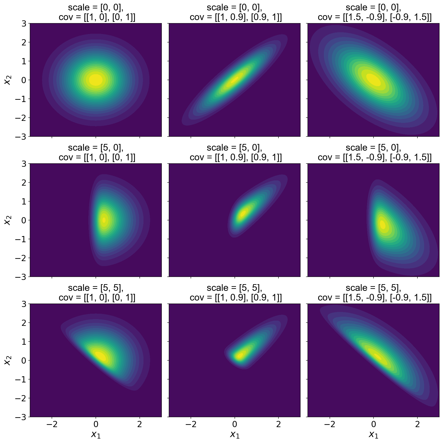
As we can see, when $\boldsymbol{\alpha}$ is a vector of zeros, the CDF evaluates to $1/2$, and Eq. $1$ reduces to a $K$-variate normal with zero mean and correlation matrix $\boldsymbol{\Omega}$. So the first rows in Figure $1$ are just multivariate normal distributions. When the first component of $\boldsymbol{\alpha}$ is positive, the first component of $\mathbf{x}$ is skewed (second row) while maintaining the correlation structure of the “underlying” Gaussian. Finally, when both values of $\boldsymbol{\alpha}$ are large, we see that both dimensions are skewed (third row). Of course, the components of $\boldsymbol{\alpha}$ can also be negative to induce negative skew.

Sampling

To sample from skew normal distribution, we could use rejection sampling. I found this idea from this StackOverflow. This is because

$2 \phi(\mathbf{x}; \mathbf{0}, \mathbf{I}) \Phi(\boldsymbol{\alpha}^{\top} \mathbf{x}) \leq 2 \phi(\mathbf{x}; \mathbf{0}, \mathbf{I}), \tag{2}$

since $\Phi(\mathbf{x})$ is a CDF and therefore in the range $[0, 1]$. In other words, we simply sample from the a spherical Gaussian and then reject if that sample is larger than $2 \phi_K(\mathbf{x})$. We can extend the previous class with the following method:

def rvs_slow(self, size=1):
    std_mvn = mvn(np.zeros(self.dim),
                  np.eye(self.dim))
    x       = np.empty((size, self.dim))
    
    # Apply rejection sampling.
    n_samples = 0
    while n_samples < size:
        z = std_mvn.rvs(size=1)
        u = np.random.uniform(0, 2*std_mvn.pdf(z))
        if not u > self.pdf(z):
            x[n_samples] = z
            n_samples += 1
    
    # Rescale based on correlation matrix.
    chol = np.linalg.cholesky(self.cov)
    x = (chol @ x.T).T
    
    return x

However, this approach is slow, and there is a faster way to sample. In (Azzalini & Capitanio, 1999), the authors propose the following. First, let

$\begin{aligned} \begin{bmatrix} x_0 \\ \mathbf{x} \end{bmatrix} &\sim \mathcal{N}_{K+1} \left( \mathbf{0}, \begin{bmatrix} 1 & \boldsymbol{\delta}^{\top} \\ \boldsymbol{\delta} & \boldsymbol{\Omega} \end{bmatrix} \right), \\ \boldsymbol{\delta} &\triangleq \frac{1}{\sqrt{1 + \boldsymbol{\alpha}^{\top} \boldsymbol{\Omega} \boldsymbol{\alpha}}} \boldsymbol{\Omega \alpha}. \end{aligned} \tag{3}$

Then if define $\mathbf{z}$ as

$\mathbf{z} = \begin{cases} \mathbf{x} & \text{if $x_0 > 0$} \\ -\mathbf{x} & \text{otherwise.} \end{cases} \tag{4}$

Then $\mathbf{z}$ is skew normal with shape $\boldsymbol{\alpha}$ and correlation matrix $\boldsymbol{\Omega}$. Since we never reject a sample, this can be easily vectorized:

def rvs_fast(self, size=1):
    aCa      = self.shape @ self.cov @ self.shape
    delta    = (1 / np.sqrt(1 + aCa)) * self.cov @ self.shape
    cov_star = np.block([[np.ones(1),     delta],
                         [delta[:, None], self.cov]])
    x        = mvn(np.zeros(self.dim+1), cov_star).rvs(size)
    x0, x1   = x[:, 0], x[:, 1:]
    inds     = x0 <= 0
    x1[inds] = -1 * x1[inds]
    return x1

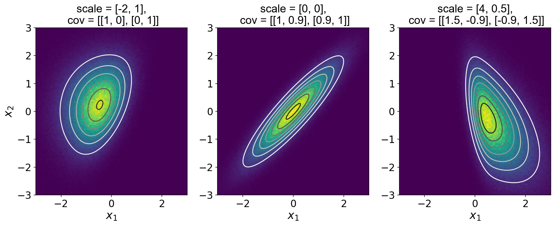
To verify this code, I generated Figure $2$, which plots one million samples from a few different skew normal distributions along with the groundtruth PDF.

Figure 2. Histograms of one million samples from three multivariate skew normal distributions with varying parameters.