The Unscented Transform

The unscented transform (UT) was originally prosed by Jeffrey Uhlmann as part of his PhD thesis (Uhlmann, 1995), although it is most well-known as a component in the unscented Kalman filter (Julier & Uhlmann, 1997; Wan & Van Der Merwe, 2000). The basic premise of the UT is that it easier to approximate a Gaussian distribution than it is to approximate an arbitrary density after a nonlinear transformation. This is a surprisingly simple and useful idea.

Imagine you have some $D$-dimensional Gaussian distributed variables,

$\mathbf{x}_n \stackrel{\texttt{iid}}{\sim} \mathcal{N}_D(\boldsymbol{\mu}_X, \boldsymbol{\Sigma}_X), \tag{1}$

you and want to estimate their density after applying a nonlinear transformation to them:

$\mathbf{y}_n = f(\mathbf{x}_n). \tag{2}$

How would we do this? If the transformation were linear, such as

$\mathbf{y}_n = \mathbf{A} \mathbf{x}_n + \mathbf{b}, \tag{3}$

this would be easy, since an affine transformation of a Gaussian is also a Gaussian. We could estimate the density of $\mathbf{y}_n$ in closed form. This is one reason why so many probabilistic models rely on linear-Gaussian assumptions (Roweis & Ghahramani, 1999). For example, in a Kalman filter, we might have some state estimation that we posit is Gaussian distributed. Linear dynamics means we propogate that estimation—and our model uncertainty—forward in time using a linear map. However, it’s less obvious what to do in Eq. $2$, when our transformation is nonlinear.

Figure 1. (Left) One thousand data points $\mathbf{X}$ (gray), as well as their sigma points (black "X" marks) and a contour plot of the Gaussian density estimated from $\mathbf{X}$. (Right) The transformed data points $\mathbf{Y} = f(\mathbf{X})$, as well as the transformed sigma points. The contour plot of the estimated Gaussian is computed only from the sigma points. The nonlinear function $f(\cdot)$ is the logistic sigmoid function.

The UT is the following: compute a subset of points, called sigma points $\mathbf{S} = \{\mathbf{s}_i\}_{i=1}^{2D+1}$, and propogate them through the nonlinear map $f(\cdot)$. Then estimate a Gaussian distribution as

$\begin{aligned} \mathbf{y}_i &= f(\mathbf{s}_i), \quad \forall i \in \{1, \dots, 2D+1\}, \\ \mathbf{y}_i &\sim \mathcal{N}(\tilde{\boldsymbol{\mu}}_Y, \tilde{\boldsymbol{\Sigma}}_Y), \end{aligned} \tag{4}$

where $\tilde{\boldsymbol{\mu}}_Y$ and $\tilde{\boldsymbol{\Sigma}}_Y$ are the sample mean and covariance, respectively. Imagine that this worked; it would be nice because it is relatively cheap, since there are only $2D+1$ sigma points. This scales well w.r.t. the dimensions of our data, compared to other methods such as Monte Carlo sampling. While there are different proposals for how to choose sigma points, let’s use the simplest one, proposed by Uhlmann in his PhD thesis.

First, let $\mathbf{L}$ denote the scaled Cholesky decomposition of the covariance matrix of $\boldsymbol{\Sigma}_X$ or

$\mathbf{L} = \text{cholesky}\left(D \boldsymbol{\Sigma}_X\right). \tag{5}$

Then the sigma points are

$\begin{aligned} \mathbf{s}_0 &= \boldsymbol{\mu}_X, \\ \mathbf{s}_i &= \boldsymbol{\mu}_X + \mathbf{L}_{:,i}, \quad \forall i \in \{1, \dots, D\}, \\ \mathbf{s}_j &= \boldsymbol{\mu}_X - \mathbf{L}_{:,j}, \quad \forall j \in \{D+1, \dots, 2D\}. \end{aligned} \tag{6}$

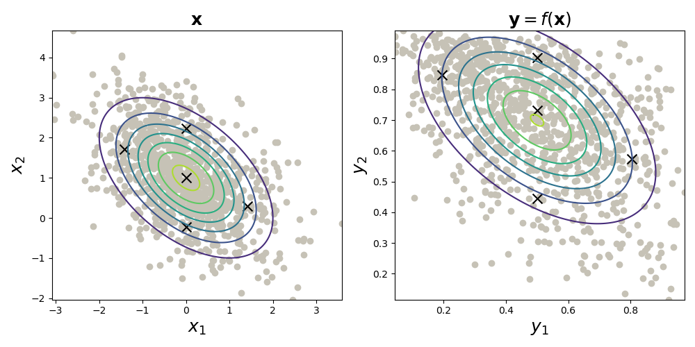
What is this doing? Speaking loosely, a positive definite matrix can be thought of as a multidimensional generalization of a positive number, and the Cholesky decomposition is then a multidimensional generalization of the square root. So we’re taking the square root of our unscaled covariance matrix, i.e. computing a multidimensional standard deviation. Eq. $6$ says that our sigma points are the sample mean of $\mathbf{X} = \{\mathbf{x}_n\}_{n=1}^{N}$, as well as points that are one standard deviation away from that mean in both directions in all dimensions $D$. This is why there are $2D + 1$ sigma points.

While that’s a mouthful, it’s easy to visualize (Fig. $1$, left). And to estimate a Gaussian density, we simply take the sample mean and sample covariance of $f(\mathbf{S})$ (Fig. $1$, right). Here, I’ve used the logistic sigmoid function for $f(\cdot)$.

That’s it. That’s the essence of the UT. There are natural extensions to this idea, such as different ways of computing the sigma points; weighting the sigma points after transforming them; and using this method to estimate non-Gaussian densities. But I think Fig. $1$ nicely captures the main idea.