Can Linear Models Overfit?

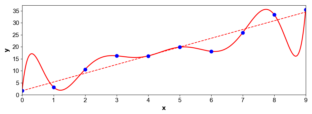
If you’re reading this, you probably already know what overfitting means in statistics and machine learning. Overfitting occurs when a model too closely corresponds to training data and thereby fails to generalize on test data. The classic example of this is fitting a high-degree polynomial to linear data (Figure $1$). Most likely, the high-degree polynomial will have high error on the next data point even though it perfectly fits the training data. One way to think about overfitting is that we have a model that is too complex for the problem, and this complexity allows the model to fit to random noise.

Figure 1. A nine-degree polynomial (solid red line) and a linear model (dashed red line) are fit to data.

A model that overfits does not adhere to Occam’s razor in its explanation of the data. I think of conspiracy theories as a good example of humans overfitting to data. For example, consider the following conspiracy theory:

Theory: John F. Kennedy was assassinated by aliens.

Is this possible? Sure. So what’s wrong with the theory? Why don’t most people believe this? The theory could be true, but one needs more evidence than is required for simpler explanations, such as that Kennedy was assassinated by Lee Harvey Oswald. Put differently, the alien explanation is more complex than the data we have. If your mental model of the world allows for highly improbable events, you can easily overfit to random noise.

The question I want to address in this post is: can a linear model overfit to data? This will motivate future posts on techniques such as Bayesian priors, Tikhonov regularization, and Lasso.

Overfitting in linear models

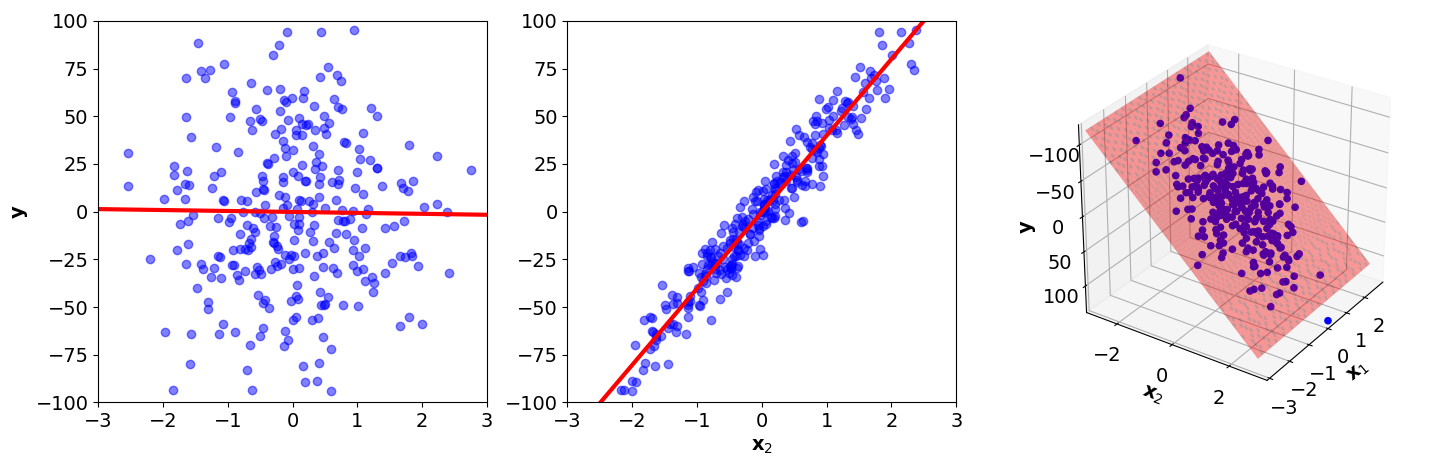
Consider fitting classical linear regression to 2D data $\{\mathbf{x}_n\}_{n=1}^{N}$ in which $x_1$ is uninformative random noise; it is completely uncorrelated with the response values $\{y_n\}_{n=1}^{N}$. Our linear model is

$y_n = \beta_1 x_{n, 1} + \beta_2 x_{n, 2} + \varepsilon_n.$

Importantly, we are assuming this model is too complex because the true $\beta_1$ is zero. So while the model in Figure $2$ visually looks okay—the linear hyperplane fits to the data quite well—it still exhibits the same kind of overfitting as in Figure $1$. Why? The model is more complex than it needs to be and thereby fits to noise. If we look at the coefficients, we can see this quantitatively:

$\beta_1 = -0.0496, \qquad \beta_2 = 40.0553.$

In Figure $2$, I’ve also drawn the planes defined by just $\beta_1$ and just $\beta_2$ to demonstrate that while $\beta_1$ should be zero, it is not. The ability of this model to generalize will be worse than if $\beta_1$ were zero.

Figure 2. A linear model fit to two-dimensional data. (Left) The response $y$ as a function of $x_1$. The marginal hyperplane defined by $\beta_1$ is shown as a solid red line. (Middle) Same as the left plot but for $x_2$. (Right) The response $y$ as a function of both $x_1$ and $x_2$. The hyperplane defined by $\boldsymbol{\beta}$ is drawn in red.

Shrinkage and priors

Understanding overfitting in linear models—understanding that certain coefficients should be smaller because they just explain noise—motivates regularizing techniques such as shrinkage and Bayesian priors. In my mind, regularization is the process of adding constraints to an under-constrained problem. For example, both convolutional filters (shared weights) in deep neural networks and an $\ell_1$ penalty on the weights of a model are regularizers. They introduce some inductive bias into the problem so that it is easier to solve.

In linear models, two common forms of regularization are shrinkage methods and Bayesian priors. In shrinkage methods such as Lasso (Tibshirani, 1996) and ridge regression (Tikhonov, 1943), large weights are penalized. We can think of this as encouraging the model to be biased towards small coefficients. A Bayesian prior such as a zero-centered normal distribution on the weights achieves a similar goal: the data must overwhelm the noise. I will discuss these techniques in future posts.