From Convolution to Neural Network

Introduction

In learning about convolutional neural networks (CNNs), I read a number of articles, blog posts, and lecture slides, most of which focused on CNNs’ distinct properties such as their architecture, shared weights, or sparse connectivity. My aim is to build up to these properties from ideas that are, at least in my experience, less thoroughly explained: what is a convolution, how is it related to image processing, and how do CNNs implement convolutions? I’ll also mention the benefits of pooling.

Convolutional neural networks: what and why?

Recall that a neural network (NN) is a hierarchical network of computational units or “neurons” for highly nonlinear function approximation. Each neuron’s input is a set of weighted upstream signals. The neuron treats this set of weighted inputs as a linear combination and optionally applies a nonlinearity.

CNNs are neural networks with a special structure that allows them to efficiently and robustly detect visual patterns in images (LeCun & others, 2015). To see why we might want a specialized neural network, consider a fully connected NN with an input of RGB color images. If each image is $3 \times 256 \times 256$ pixels ($3$ for the number of color channels), then a single neuron in the first fully connected hidden layer would have $196,608$ weights. This is a lot. CNNs make a few simplifying assumptions about images and thereby dramatically reduce the number of learnable parameters. In this context, CNNs can be viewed as a kind of regularized NN.

Convolutions and kernels

As their name suggests, the distinguishing idea behind convolutional neural networks is the convolution, which is related to the idea of a kernel. After understanding convolutions and kernels, the special structure of CNNs will make more sense.

Discrete convolutions in 1D

A convolution is a mathematical operation on two functions that outputs a function that is a modification of the two inputs. Since it is sufficient for our purposes, I will only discuss the discrete convolution operator, but Goodfellow et al (Goodfellow et al., 2016) has a broader discussion. A discrete convolution between two single-variable functions $f$ and $g$, denoted with an asterisk ($*$), is defined as:

$(f * g)(x) \triangleq \sum_{i=-\infty}^{\infty} f(i) \cdot g(x-i)$

My intuition is that we are “sliding” the function $g$ across the function $f$ and outputting a new function in the process. To see this, let’s work through an example. Imagine we have a 1D input signal representing an audio recording with white noise, and we want to eliminate the noise. We can use the convolution operation to do this to do this. Our input signal is a sequence of numbers:

$f = [10, 9, 10, 9, 10, 1, 10, 9, 10, 8]$

To be clear, the function $f$ is a mapping from a time point (the index of the list) to a signal value. Using the ordered-pair notation for a function:

$f = \{(0, 10), (1, 9), (2, 10), (3, 9), (4, 10), (5, 1), (6, 10), (7, 9), (8, 10), (9, 8)\}$

Here is a plot of the signal:

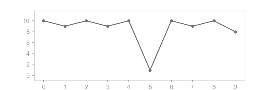
If we want to smooth this signal to eliminate deviations like $f(5) = 1$, then we can define our second function $g$, the kernel, as the following:

$g = \left[\frac{1}{3}, \frac{1}{3}, \frac{1}{3} \right]$

Before reading further, stop and think about what this second function will do to the first once they are convolved. To see the effect, let’s convolve for a few time points, starting with $x = 0$:

$y(0) = \sum_{i=-\infty}^{\infty} f(i) \cdot g(0-i)$

While this is a summation from negative to positive infinity, notice that most values are undefined. $f$ is only defined for nonnegative $i$, and $g$ is only defined when $0 \leq x-i \leq 2$. We omit these undefined terms (or define them as $0$) and get:

$\begin{aligned} y(0) &= f(0)g(0) &&= 10 \cdot \frac{1}{3} &= 3 \frac{1}{3} \\ y(1) &= f(0)g(1) + f(1)g(0) &&= 10 \cdot \frac{1}{3} + 9 \cdot \frac{1}{3} &= 6 \frac{1}{3} \\ y(2) &= f(0)g(2) + f(1)g(1) + f(2)g(0) &&= 10 \cdot \frac{1}{3} + 9 \cdot \frac{1}{3} + 10 \cdot \frac{1}{3} &= 9 \frac{2}{3} \\ y(3) &= f(1)g(2) + f(2)g(1) + f(3)g(0) &&= 9 \cdot \frac{1}{3} + 10 \cdot \frac{1}{3} + 9 \cdot \frac{1}{3} &= 9 \frac{1}{3} \end{aligned}$

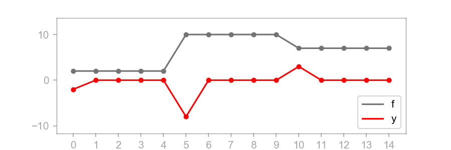
Here is a plot of the original signal $f$ and the output function $y$:

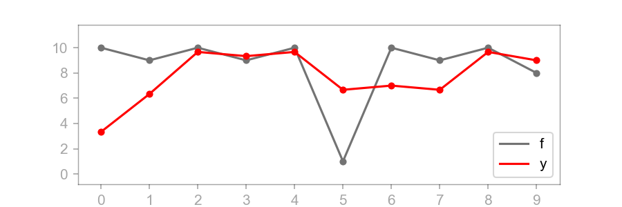
Visually, we can see that $y$ is a smoothed version of $f$. The plot of $y$ begins at $3.\overline{3}$ because $g$ is only smoothing one data point. But once $x = 2$, $g$ sums three elements of $f$ and then divides by $3$, i.e. computes the average. Once $f(5) = 1$ is encountered, $y$ dips but not as extremely as $f$. It takes three time steps for the effects of $f(5)$ to disappear from $y$. This is because the size of $g$’s domain is three.

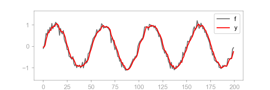
This effect is more clear on a larger scale. For example, in the image below $g$ is convolved with a noisy sine wave:

An attentive reader might have noticed that the convolution operation inverts $g$ before multiplying element-wise and summing; the pattern when $k$ is the number of elements in $g$ is:

$y(x) = f(x - (k-1))g(k-1) + f(x-k)g(k-2) + \ldots + f(x)g(0)$

Why is this flipped? There are some interesting reasons for this, but it is beyond the scope of this post. The simplest explanation is this: that’s the definition of a convolution. If we did not flip $g$, the operation would be called cross-correlation.

Finally, here is an implementation of a 1D discrete convolution in Python. I hope that given the above discussion, the code is straightforward to understand.

import matplotlib.pyplot as plt

# F and G are the two functions we want to convolve.
F = [10, 9, 10, 9, 10, 1, 10, 9, 10, 8]
G = [1./3, 1./3, 1./3]
N = len(F)
Y = range(N)

# Convolve F with G.
for x in range(N):
    total = 0
    for i in range(len(F)+1):
        if len(F) > i >= 0 and len(G) > x-i >= 0:
            total += F[i] * G[x-i]
    Y[x] = total

# Plot results.
fig, ax = plt.subplots()
time = range(N)
ax.scatter(time, F, color='gray')
ax.plot(time, F, color='gray', label='f')
ax.scatter(time, Y, color='red')
ax.plot(time, Y, color='red', label='y')
ax.legend(loc='lower right')
plt.show()

Discrete convolutions in 2D

Now let’s generalize to 2D. The equation for a 2D discrete convolution is:

$(f * g)(x_1, x_2) = \sum_{i=-\infty}^{\infty} \sum_{j=-\infty}^{\infty} f(i, j) \cdot g(x_1 - i, x_2 - j)$

For example, if $f$ and $g$ are:

$f = \begin{bmatrix} 1 & 2 & 3 & 4 & 5 \\ 6 & 7 & 8 & 9 & 10 \\ 11 & 12 & 13 & 14 & 15 \\ 16 & 17 & 18 & 19 & 20 \end{bmatrix} \quad g = \begin{bmatrix} a & b & c \\ d & e & f \\ g & h & i \end{bmatrix}$

Then to convolve $f$ with $g$ at $(1,1)$:

$(f * g)(1,1) = \sum_{i=-\infty}^{\infty} \sum_{j=-\infty}^{\infty} f(i, j) \cdot g(1 - i, 1 - j)$

$= f(0, 0)g(1, 1) + f(0, 1)g(1, 0) + f(1, 0)g(0, 1) + f(1, 1)g(0, 0)$

$= 1e + 2d + 6b + 7a$

The sum has only four terms because $f$ and $g$ are defined for only those values. Notice that $g$ has been flipped twice, once over the $x$-axis and once over the $y$-axis. (This flipping is irrelevant for kernels that are symmetric in both dimensions, but it is important to be consistent with the 1-dimensional definition.) The resulting function $y$ is also a matrix.

A succinct way to describe this is that we took the sum of the elements in the Hadamard product of two matrices:

$\text{sum}( \begin{bmatrix} 1 & 2 \\ 6 & 7 \end{bmatrix} \circ \begin{bmatrix} e & d \\ b & a \end{bmatrix} )$

Kernels

Now that we understand convolutions, we can discuss kernels. A kernel is a matrix or function used to process an image. Using the same notation as above, $f$ is a section of image and $g$ is the kernel. Kernels are useful for filtering images, for example blurring; blurring is completely analogous to smoothing in 1D. We can interpret $y$ to be a filtered version of our input image.

Now by convention, the kernel function $g$ is defined such the center cell is $(0,0)$. Using this convention on the matrices above, we get a different sum because $g$ is defined for $[-1, 1]$ for both axes:

$\begin{aligned} (f * g)(1,1) &= f(0, 0)g(1, 1) + f(0, 1)g(1, 0) + f(0, 2)g(1, -1)\\ &+ f(1, 0)g(0, 1) + f(1, 1)g(0, 0) + f(1, 2)g(0, -1)\\ &+ f(2, 0)g(-1, 1) + f(2, 1)g(-1, 0) + f(2, 2)g(-1, -1)\\ \\ &= 1i + 2h + 3g + 4f + 5e + 6d + 7c + 8b + 9a \end{aligned}$

Also note that if the kernel were symmetric, then the operation is easier to visualize because we would just sum the Hadamard product of a section of $f$ and $g$:

$\text{sum}( \begin{bmatrix} 1 & 2 & 3 \\ 6 & 7 & 8 \\ 11 & 12 & 13 \end{bmatrix} \circ \begin{bmatrix} a & b & c \\ d & e & f \\ g & h & i \end{bmatrix} ) = 1a + 2b + 3c + 6d + 7e + 8f + 11g + 12h + 13 i$

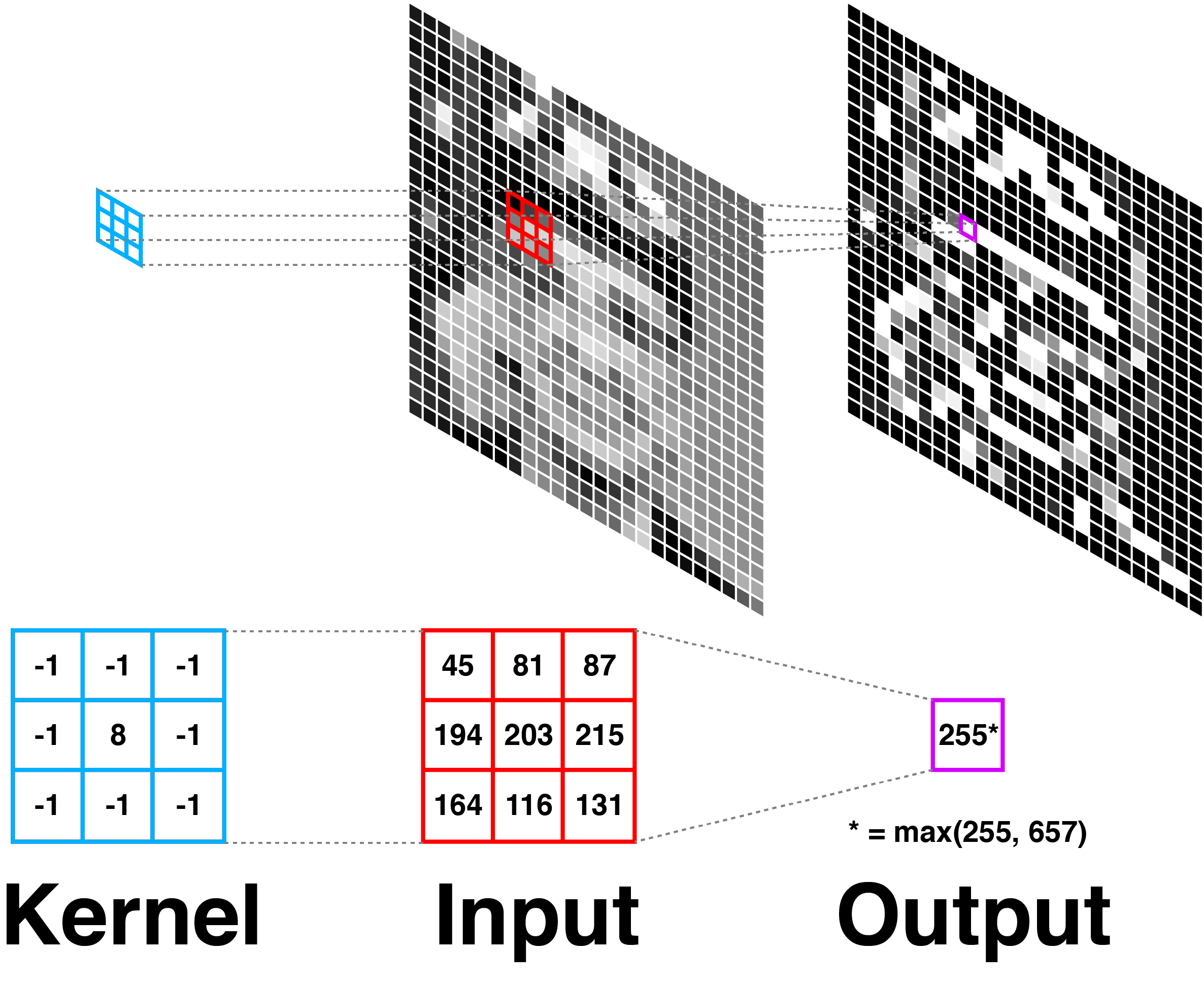
Now to see why kernels and convolutions are useful in image processing, imagine we apply the following kernel to every pixel in an image:

$\begin{bmatrix} -1 & -1 & -1 \\ -1 & 8 & -1 \\ -1 & -1 & -1 \end{bmatrix}$

The result is edge detection. If the sum of the neighbors’ values is roughly equal to the center pixel’s value, the kernel will return a number close to $0$. If there is a strong difference in pixel values in the kernel, the center will be positive. Since white is taken to be $255$ while black is taken to be $0$ by convention, this will create an image of white edges on a black field. Below, we visualize this operation applied to an image of Grace Hopper:

Notice that the kernel is applied to every pixel in an image. Often, this is described as the kernel “sliding” across the image. The visual effect of convolving a kernel with an image is what we might call “filtering.” I mean nothing deep by this word; it is the same idea as applying a filter in Photoshop or on Instagram. For example, here are are two kernels applied to slightly larger images of Hopper:

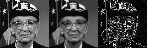From left to right: Original, blurred, edge detected.

The blur filter using the mean kernel, which is a two-dimensional version of our 1D smoothing function. The edge detection filter using the Laplace kernel, which we presented above.

Here is my Python code for the Laplace kernel:

import numpy as np
from scipy.misc import lena
from PIL import Image

SIZE = 3

# Laplace kernel
K = np.zeros((SIZE, SIZE))
center = int(np.floor(SIZE / 2))
K[:,:] = -1
K[center, center] = K.size - 1

image = np.uint8(lena())
filtered = np.zeros(image.shape)

offset = int(np.floor(SIZE / 2))
for i in range(offset, filtered.shape[0]-offset):
    for j in range(offset, filtered.shape[1]-offset):
        X = image[i - offset:i + offset + 1, j - offset:j + offset + 1]
        value = (X * K).sum()
        filtered[i, j] = min(255, max(0, value))

image = Image.fromarray(image)
image.show()
image = Image.fromarray(filtered)
image.show()

There are many types of kernels and methods to achieve the same effect. I have implemented a few kernels and put them on GitHub here.

Now that we understand kernels, we can succinctly state what CNNs do: they automatically learn kernels from image data. Given a dataset of images, a CNN will learn many different kernels in order to extract discriminating features in the images. To be clear, these kernels will probably not be like the kernels humans might design by hand.

Location invariance

This idea is visually obvious, but it is worth stating: kernels detect image features in a way that is location invariant. If a kernel detects edges, it will detect edges anywhere. If it detect red circles, it will detect red circles anywhere. This property of kernels represents an assumption about the data, but one that makes sense for images and is clearly related to how humans see the world. Later, when we discuss CNN architecture, we demonstrate how it takes fewer parameters to model this assumption (hint: shared weights).

Pooling for robustness

The second important idea behind CNNs is pooling. Pooling is very similar to downsampling and is even called that in some NN libraries. There are multiple ways to perform pooling such as max, average, and sum. This is a straightforward idea that is explained well in a variety of places, i.e. (Karpathy, 2016).

Pooling is easy to understand, but there is an important benefit that is good to visualize: pooling discards fluctuations and variances in images. This robustness to small variations is important. Note that LeCun included it in his description of CNNs (LeCun & others, 2015):

They can recognize patterns with extreme variability (such as handwritten characters), and with robustness to distortions and simple geometric transformations

I want to demonstrate this robustness using an imaginary CNN that can correctly classify MNIST digits (LeCun et al., 2010). First, imagine our CNN has learned some kernels to correctly classify the digit “$2$”. For simplicity, assume it learned a kernel identical to the Sobel operator for horizontal edges. If we convolve this kernel and then use max pooling, we get:

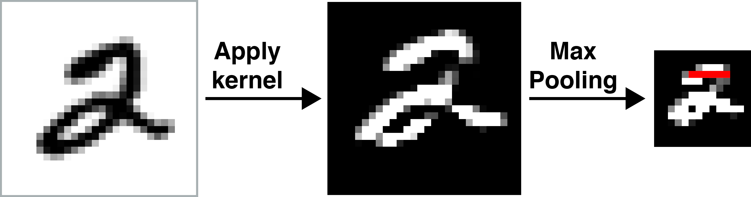
I have drawn a red horizontal bar as an imaginary indicator of “$2$”. Whenever the CNN detects that red bar, in addition to other features of “$2$”, it will classify the digit as $2$.

Next, imagine we modify the digit slightly. Below, I have edited the digit so that the top-left line in the glyph is more horizontal than before. What happens?

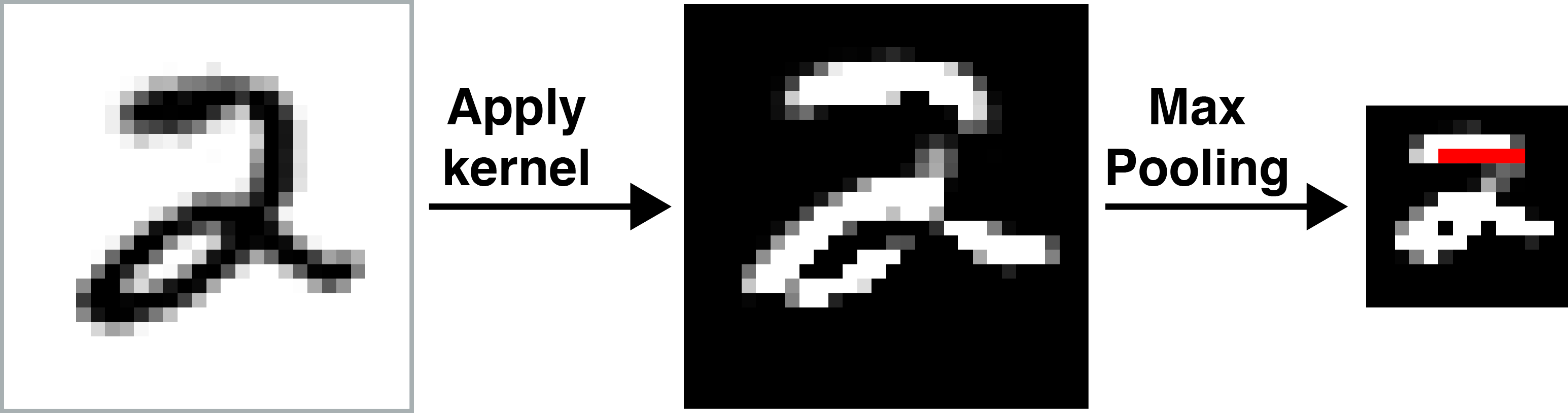
The key idea is that the red horizontal line is still there. This is what we mean by “translational invariance.” The CNN is robust to small changes to the digit. This robustness is due to pooling, not due to more samples. So we get some translational invariance for free, rather than having to train on images that are nearly identical except for small variations. By combining kernels and pooling, CNNs can detect the same feature anywhere on the visual field and are robust to small variations in the features.

Network architecture

Now that we understand kernels and pooling, we are ready to understand CNN architecture. CNNs have three types of layers: convolutional, pooling, and fully-connected. Convolutional layers learn kernels for discriminating features; pooling layers perform downsampling to compress the representation and gain some translational invariance; and the fully-connected layers are typically at the end of the network for classification.

Now given what we know so far, I think the most interesting question is: how do we implement learnable kernels in the convolutional layers? Personally, I found this connection to be the least well-explained aspect of CNNs—or at least most difficult for me to understand—so I’m going to be as explicit as possible.

Shared weights

I introduced a kernel as a small matrix which we apply to every pixel in an image. I visualize this as sliding the kernel across the image plane, convolving as we go. My example code uses for loops to do this. But once we talk about CNN architecture, the notions of “sliding” and for loops are misleading. We actually use shared weights.

Let’s demonstrate how shared weights can be used to model a kernel. To simplify things, let’s move back to 1D for now. Let our input signal $f$ be:

$f = [2, 2, 2, 2, 2, 10, 10, 10, 10, 10, 7, 7, 7, 7, 7]$

This time, our 1D kernel $g$ will detect edges:

$g = [-1, 1]$

Here is a plot of $f$ and $y = (f * g)$:

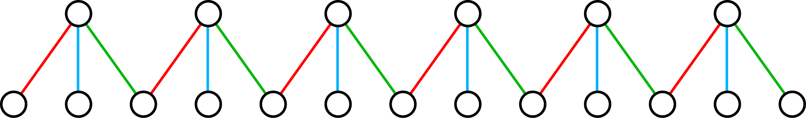
Now we can express this operation as a special kind of neural network layer in which the weights are shared. Below, I have diagrammed this. The red weights (left) are $1$ and the blue weights (right) are $-1$. Remember that the convolution operator inverts $g$:

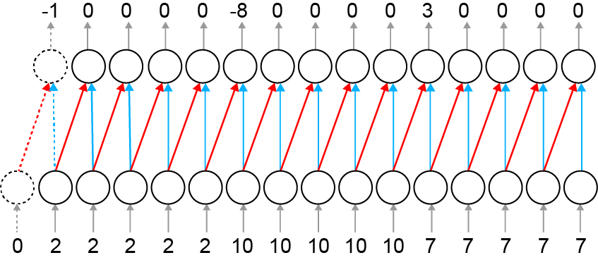The input (bottom row) is $f$; the output (top row) is $(f * g)$. Red lines have weights of $1$; blue lines have weights of $-1$

The input to the network is $f$ and the output is $y = (f * g)$. In other words, by using shared weights, we have a network layer that is functionally equivalent to convolving a 1D kernel with our input. Note that to prevent the domain of $y$ from being smaller than $f$, we can add an extra input neuron. This is called padding. In 2D, when the origin of function is in the center of the matrix, we would add the padding symmetrically.

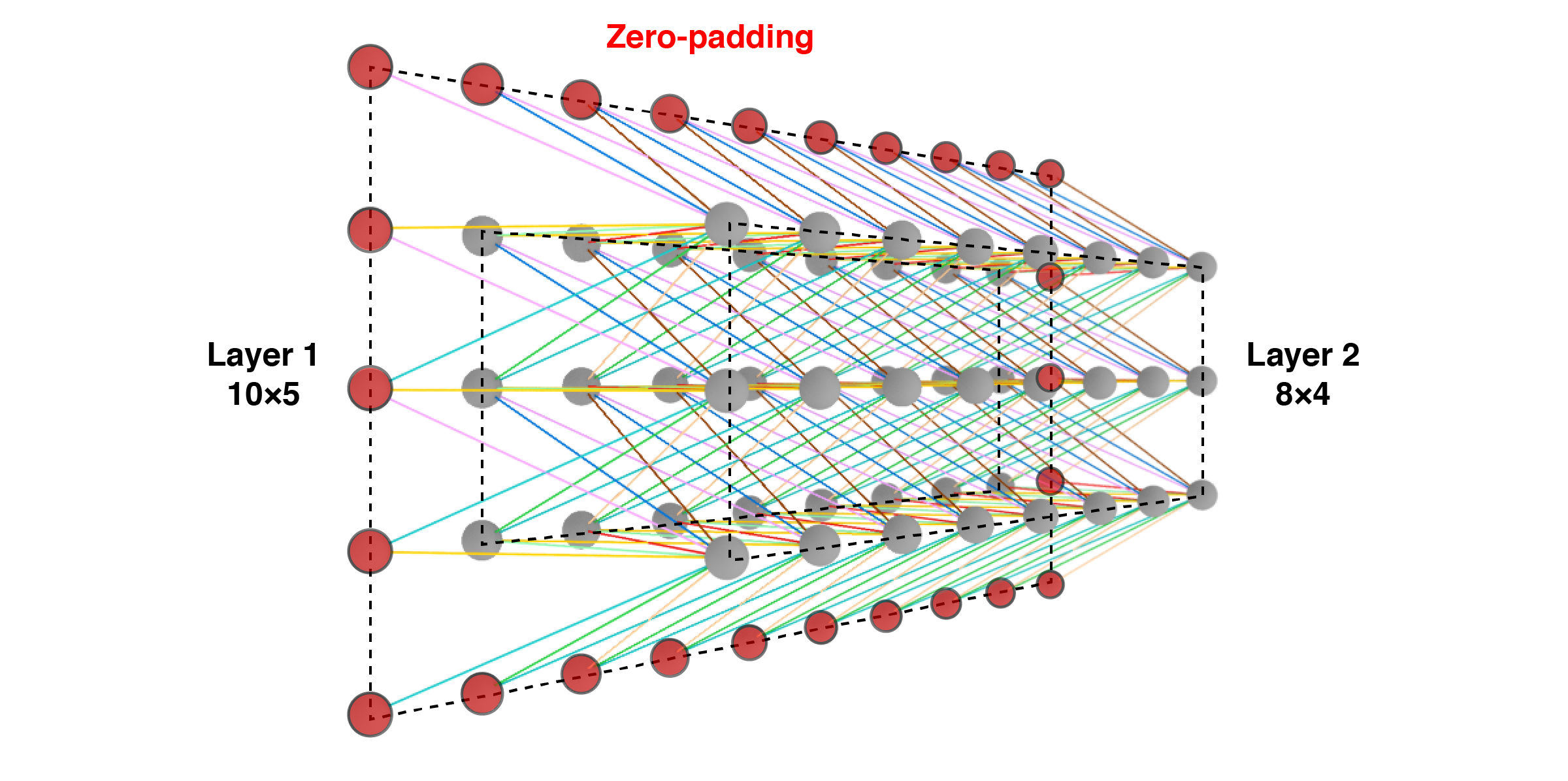
Of course, the above diagram is only for a 1D input. Below is my attempt at a visualization for a 2D input. Shared weights are the same color. The key point is that the downstream neurons (right) each take an input signal from a $N \times M$ grid (in this case, $N = M = 3$) in the previous layer. The shared weights are functionally equivalent to convolving a kernel across the entire image:

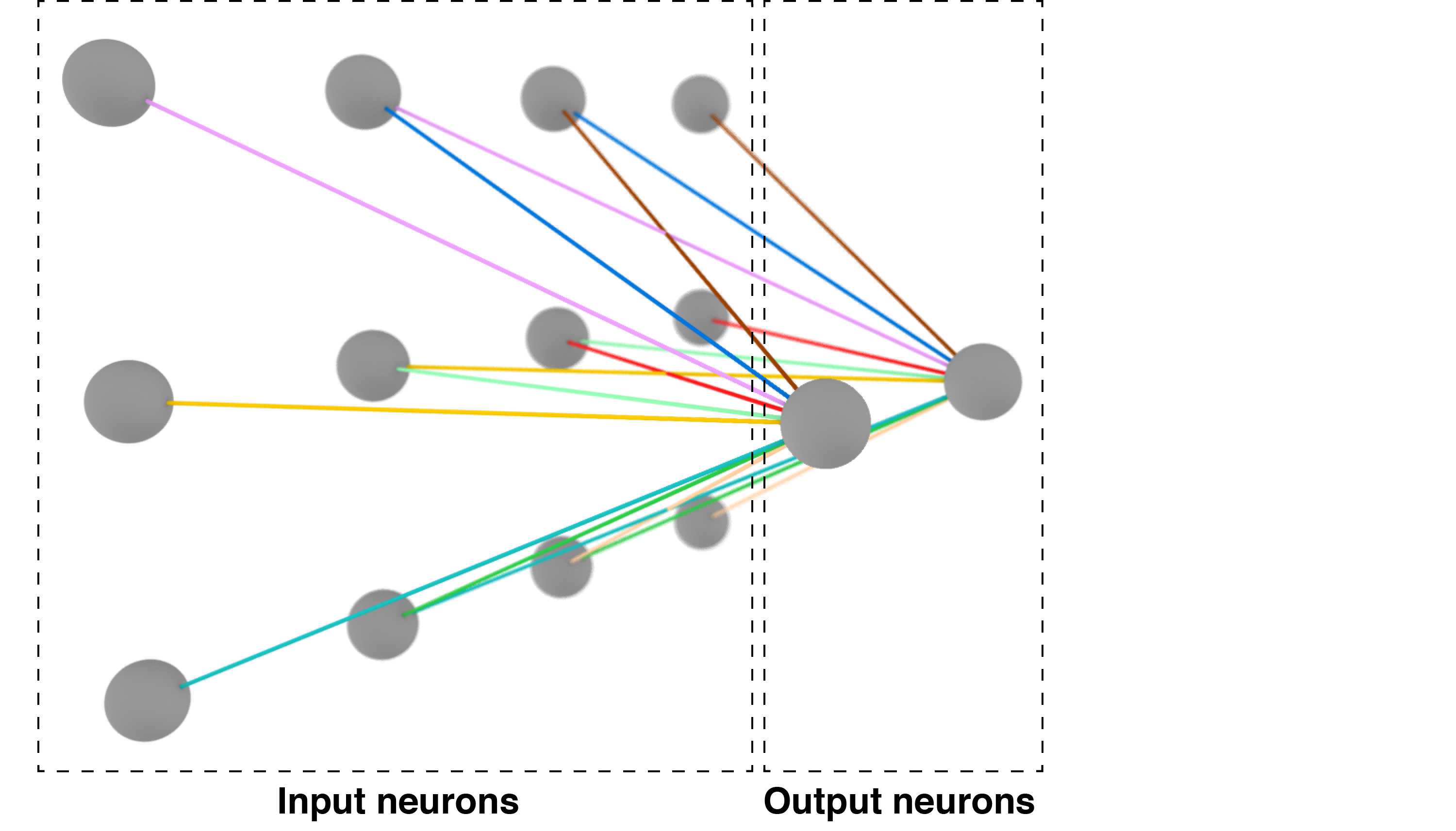Three-dimensional visualization of shared weights. Shared weights are the same color.

Shared weights also allow us to demonstrate the location invariance of kernels quantitatively. For example, below I have drawn a small convolutional layer with a nonlinear function $\sigma$ and arbitrary chosen shared weights. Observe that the output is the same, regardless of where the feature $x$ appears along the input space.

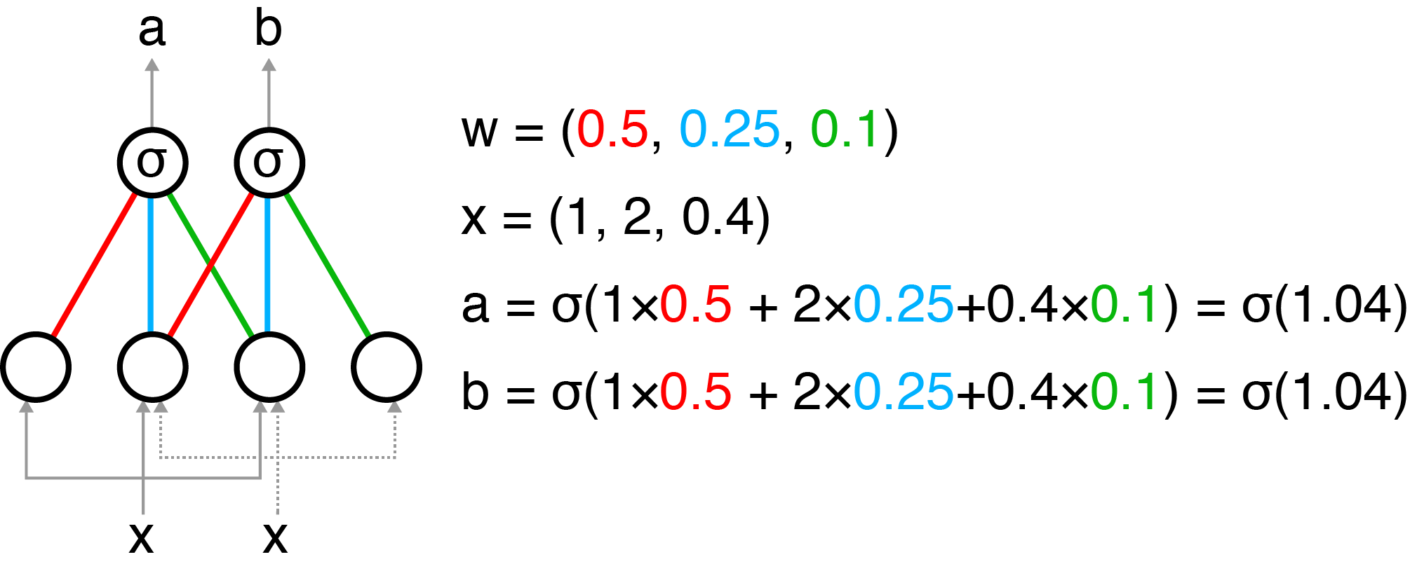
In summary, the set of shared weights that define a convolutional layer are functionally equivalent to the kernel used in traditional image processing. They allow the CNN to detect features regardless of their location in an image and reduce the number of parameters that must be learned by the network.

Layers as volumes

It would be not be particularly useful for a CNN to learn a single set of shared weights. Clearly to achieve the kind of performance that has made CNNs famous requires the ability to detect many image features. For this reason, convolutional layers are typically discussed as three-dimensional volumes of neurons. The first two dimensions are the plane of the image. The third dimension is the number of kernels that can be learned in a single convolutional layer.

This is not the easiest thing to diagram, but this is my attempt:

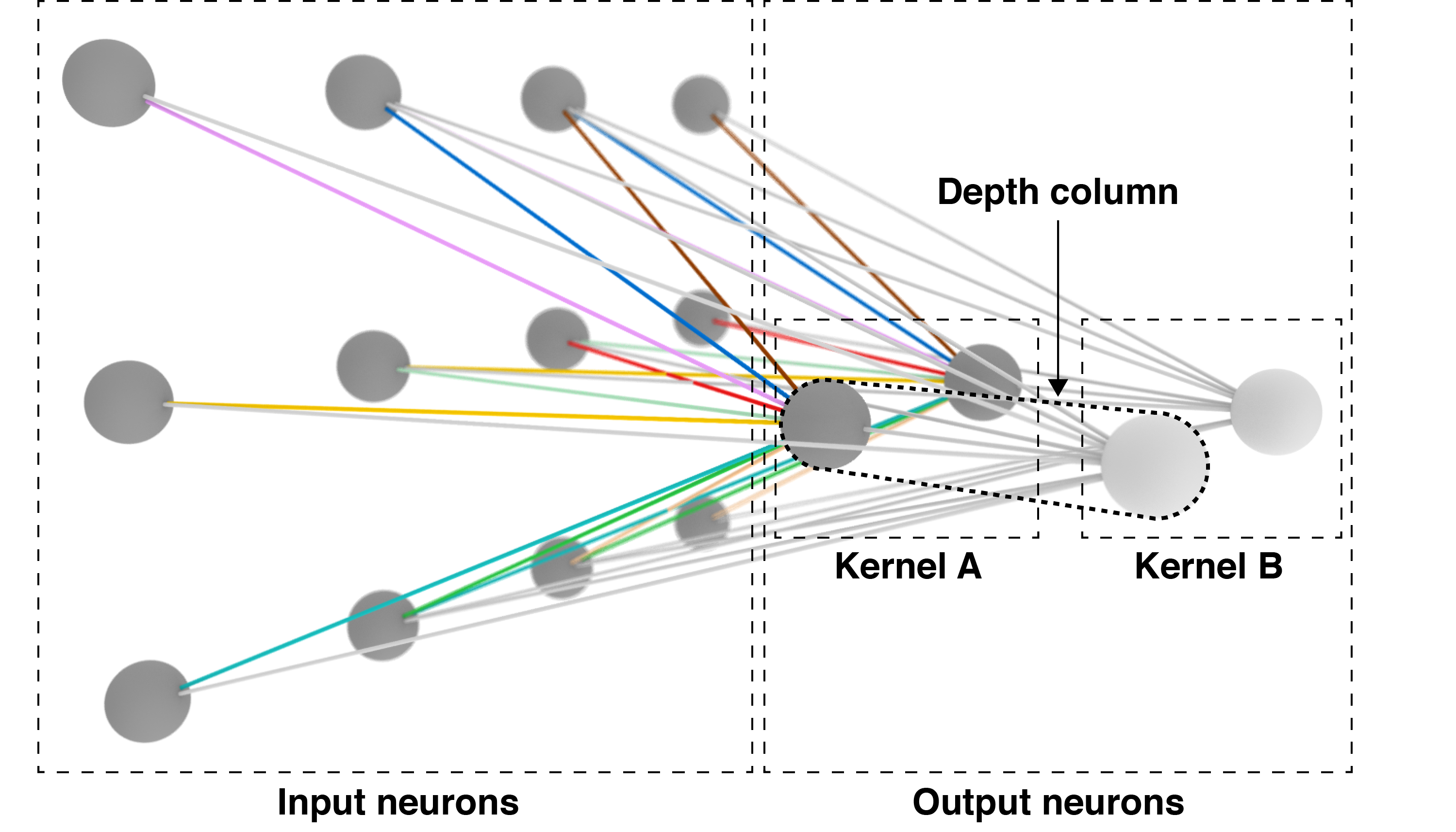Two kernels in the same convolutional layer. Kernel $B$'s weights have no color for ease of visualization.

The point is that a single convolutional layer has depth, and that depth indicates the number of kernels that can be learned by that layer. Above, we have a convolutional layer that learns two kernels. The set of neurons all connected to the same region of input is called the depth column.

Importantly, RGB images have three “layers” of values. Therefore, the input to a CNN is often $W \times H \times 3$ where $W$ is the width, $H$ is the height, and $3$ is the depth of the image. In that case, the convolutional layer’s depth would be a fourth dimension. For simplicity and consistency, I have only discussed grayscale images. I think extending these ideas to three- and four-dimensions is clear enough.

Hyperparameters

Now that we understand CNN architecture, we can discuss the network hyperparameters. The output dimensions of a convolutional layer are dependent upon these hyperparameters, as well as the size of the input. There are four important ones:

• Receptive field ($R$): This indicates how many neurons in a convolutional layer are connected to a single output neuron, i.e. how big is the kernel. For example, in the 3D rendering above, the receiptive field is $3 \times 3$.

• Depth ($D$): This corresponds to the number of kernels we want to learn in a single convolutional layer or the size of the depth column.

• Stride ($S$): This corresponds to how frequently the shared weights are repeated. This is functionally equivalent to the step size if we were sliding the kernel across the image. For example, when the stride is $3$, we “move” the kernel $3$ pixel at a time. Just remember that “move” or “step” is misleading. We are actually repeating the tiling of shared weights.

• Zero-padding ($P$): This specifies extra neurons with zeros as input to ensure that the output and input are the same size. Otherwise, the output of a convolutional layer may be smaller than the input. For example, here is a convolutional layer with a $3 \times 3$ receptive field that takes as input a $10 \times 5$ image. Notice that the output is only $8 \times 3$. If we wanted the output to be the same size as the input, we would need zero-padding of 1 on all sides:

There is a simple equation to compute the size of the output given these hyperparameters. This equation works for width ($O_w$) or height ($O_h$). I’ll just use width as an example:

$O_w = \frac{I_w - R_w + 2P_w}{S} + 1$

Why does this equation work? We subtract $R_w$ because we are actually subtract half of $R_w$ on each side. We add $2P$ because we are adding full padding to each side. We divide by $S$ to get how many strides we can fit given the number of neurons. And $+1$ because of fence posts.

For example, let $I = 13$, $F=3$, $P=0$, and $S=2$. Then:

$\frac{13 - 3 + 2(0)}{2} + 1 = 6$

If we draw this as a sanity check, we get:

Which looks correct.

The output depth $O_d$ is flexible. See the section Layers as volumes above for why.

It is worth mentioning that it is possible to have impossible configurations. For example, what if the input width is $10$, padding is $0$, and kernel size is $3$? In my opinion, a good library should throw an exception, but they can fail silently. My guess is that sizing CNNs is the source of headaches for many beginners.

Conclusion

Convolutional neural networks are specialized neural networks for detecting visual patterns and features from images. They recognize features regardless of their location in the image, and with pooling they are robust to small variances. They work by automatically learning kernels or sets of shared weights for feature detection.