Approximating Stirling's Approximation

I have always been slightly uncomfortable with Stirling’s approximation of the factorial:

$n! \simeq \sqrt{2 \pi n} \left( \frac{n}{e} \right)^n. \tag{1}$

I was uncomfortable because it just felt like magic. Sure, I could read a proof that shows it is true, but why does it work? How did Stirling come up with it? Could I have reasoned my way to this approximation on my own?

But after learning more about the history of the approximation (Dutka, 1991), I found this relationship a bit less mysterious. In fact, I think the history of this problem is a great example of street-fighting mathematics—that is, using basic mathematics, approximations, and guesswork to reason quantitatively, rather than using exact proofs.

So the goal of this post is not to prove that Stirling’s approximation is true. The goal of this post is to use basic mathematics to show it is plausible. In my mind, this was probably how early mathematicians such as Abraham de Moivre and James Stirling approached this problem. Long before they could prove that Equation $1$ was true, they had to have somehow convinced themselves that it or a similar functional form were likely. So let’s try to retrace some early steps to gain the same conviction.

Perhaps the most fundamental insight needed is that it is often easier to deal with sums rather than products; and so rather than thinking about $n!$, let’s think about its log:

$\log\!\left(n!\right) = \sum_{i=1}^{n} \log i. \tag{2}$

This looks a lot like a Riemann integral with a sub-interval width $\Delta x = 1$, which is an approximation of the integral of $\log (x)$ (Figure $1$).

Figure 1. A Riemann integral with $\Delta x = 1$ approximating the integral of $\log(x)$.

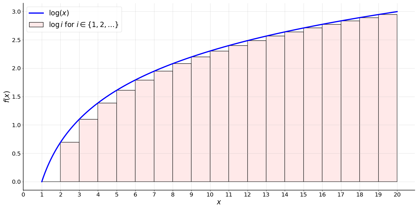
And so we already have a spark of hope, because integrals sometimes have nice, closed forms. So our very first guess might be this:

$\sum_{i=1}^{n} \log i \approx \int_1^n \log(x) dx. \tag{3}$

Conveniently, we can solve this integral using integration by parts:

$\int_1^n \log(x) dx = n \log n - n + 1, \tag{4}$

and this gives us our first approximation:

$\log(n!) \approx n \log n - n + 1. \tag{5}$

If we exponentiate both sides, we get something very promising:

$n! \approx g(n) := e \left( \frac{n}{e} \right)^n. \tag{6}$

Furthermore, notice that since $25^2 = 625$, then

$\sqrt{2\pi} \approx \sqrt{6.28} \approx 2.5 \approx e. \tag{7}$

So with nothing more than elementary calculus and napkin math, we have an approximation that appears to be within a factor of $\sqrt{n}$.

But of course, if we’re early mathematicians, it might not be obvious that this is promising because we don’t know Equation $1$ a priori. What could we do? We could check if we’re onto something by computing both $n!$ and $g(n)$ for increasing values of $n$. Luckily for us, we have computers, but since $n!$ grows very, very quickly, it is hard to visualize. The last datum always dominates $y$-axis. So instead, I’ve plotted the ratio between $n!$ and $g(n)$. This ratio should be easy to visualize since it does not grow exponentially (Figure $2$).

Figure 2. The ratio between $n!$ and $g(n)$, where $g(n)$ is defined in Equation $6$.

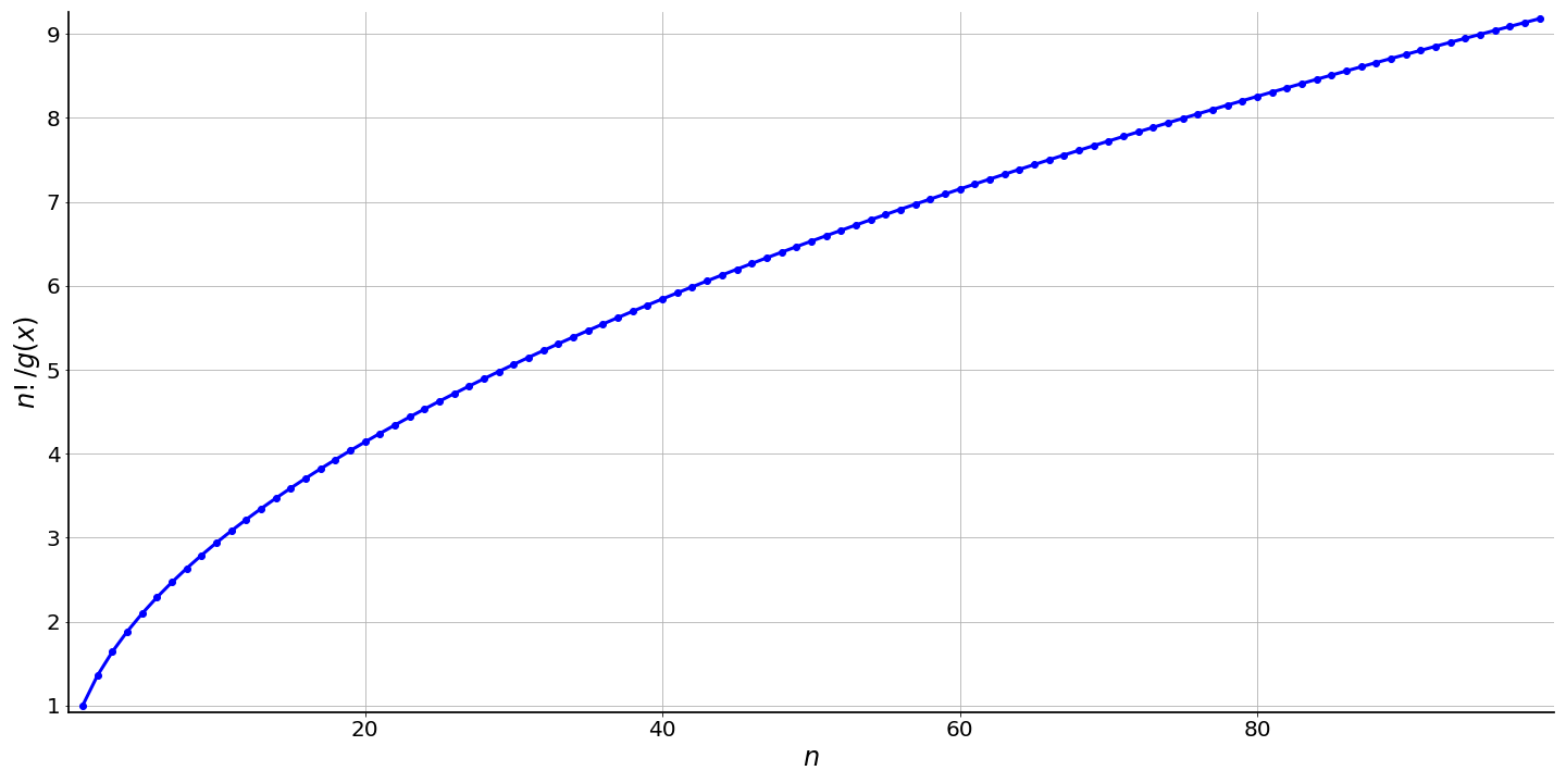
Using Heron’s method for estimating square roots in our head, we can quickly check that this ratio grows roughly with $\sqrt{n}$:

$\begin{aligned} \sqrt{20} &\approx 4.5^2, \\ \sqrt{40} &\approx 6.3^2, \\ \sqrt{60} &\approx 7.5^2, \\ \sqrt{80} &\approx 9^2, \\ &\dots \end{aligned} \tag{8}$

In other words, this figure is screaming at us that our approximation is missing a factor proportional to $\sqrt{n}$. Of course it is. I very conveniently plotted the one ratio that would highlight this fact. But let’s pretend we didn’t know this. Could we have gotten to $\sqrt{n}$ another way?

In fact, we can derive $\sqrt{n}$ using just a little more calculus. Recall the trapezoidal rule for approximating integrals. We can approximate a definite integral with endpoints $a$ and $b$ as

$\int_a^b f(x) dx \approx \frac{\Delta x}{2}\left( f(x_0) + 2f(x_1) + 2f(x_2) + \dots + 2f(x_{n-1}) + f(x_n) \right), \tag{9}$

where the points $\{x_i\}$ partition the region with a constant sub-interval width $\Delta x$. The basic idea is that we’re approximating each sub-interval of the Riemann integral with a trapezoid rather than a rectangle. This introduces many $0.5 f(x_i)$ terms, due to the triangular”tops”.

Figure 3. An approximation of the integral $\log (x)$ using the Trapezoidal rule. Here, this is a Riemann integral with $\Delta x = 1$ plus additional triangles to lower the approximation error.

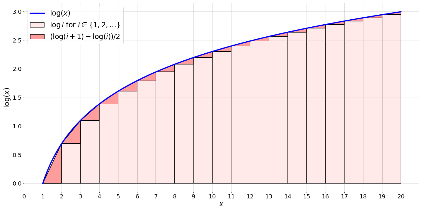
Each intermediate $0.5 f(x_i)$ term has a “sibling” such that the pair sums to unity. The only two terms which don’t have a sibling are at the endpoints $a := x_0$ and $b := x_n$.

So a second key insight is to realize that the right-hand side of Equation $2$ is essentially this integral approximation using the trapezoidal rule, except for an extra $0.5 f(x_i)$ for the two endpoints! In other words, we can refine our integral approximation as:

$\sum_{i=1}^n \log i - \frac{1}{2}\left( \log 1 + \log n \right) \approx \int_0^n \log(x) dx. \tag{10}$

Combining this with Equation $4$, we get

$\log n! \approx n \log n - n + 1 + \frac{1}{2} \log n. \tag{11}$

And exponentiating both sides, we can derive an approximation that is very close in spirit to Stirling’s approximation:

$n! \approx h(x) := e \sqrt{n} \left( \frac{n}{e} \right)^n. \tag{12}$

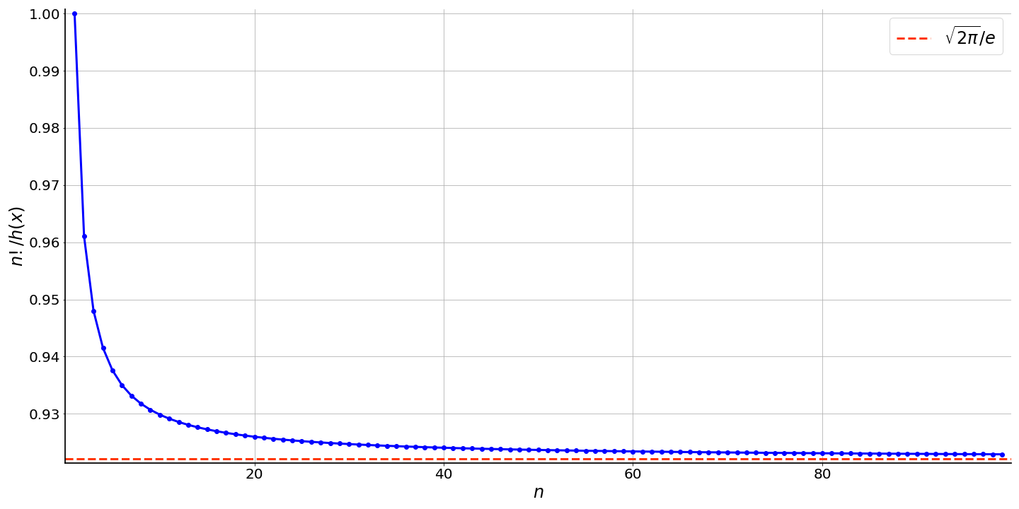
Now we’re only off from the true approximation by a constant factor,

$\frac{\sqrt{2 \pi}}{e} \approx 0.92. \tag{13}$

This is not a function of $n$, so if we plot the ratio $n! / h(n)$, we should expect the ratio to rapidly decay to this factor, which it does (Figure $4$).

Figure 4. The ratio between $n!$ and $h(n)$, where $h(n)$ is defined in Equation $12$.

So that’s it. With some basic calculus and plausible reasoning, we were able to derive an approximation of $n!$ that is quite close to true approximation discovered by de Moivre and Stirling. Of course, the reasoning here does not constitute a proof, but in my imagination, this kind of thinking might have guided someone through a more rigorous process. In fact, my understanding is that Stirling is credited with this approximation precisely because he proved the missing factor $\sqrt{2 \pi}$. So mathematicians knew some form of this approximation was plausible well before Stirling made it rigorous.

Perhaps the most interesting question now might be: why does the number $\pi$ come into an asymptotic approximation of $n$ factorial? This is an interesting question, but it is big enough to warrant a second post. Thankfully, I don’t need to write that, since Donald Knuth has already given an interesting talk on just this question: Why Pi?