Expectation of the Truncated Lognormal Distribution

Consider a random variable $Y$ which is lognormally distributed with parameters $\mu$ and $\sigma$:

$Y = \exp(X), \qquad X \sim \mathcal{N}(\mu, \sigma^2). \tag{1}$

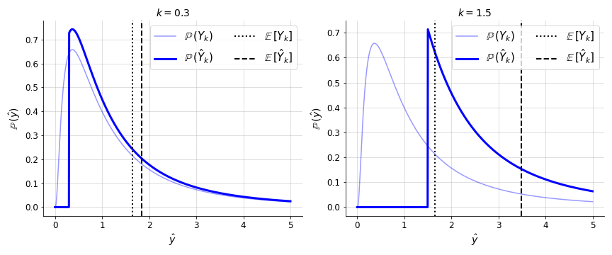
Now consider the left-truncated variable $\hat{Y}$, defined as

$\hat{Y} = \begin{cases} Y & \text{if $Y \geq k \gt 0$,} \\ 0 & \text{else.} \end{cases} \tag{2}$

The goal of this post is to derive the expected value of $\hat{Y}$. Intuitively, we might expect this value to be greater than the expected value of $Y$, since left-truncation eliminates probability mass in the left tail of the distribution (Figure $1$).

Figure 1. The probability density function of a random variable which is lognormally distributed with parameters $\mu = 0$ and $\sigma = 1$ and then truncated at $k = 0.3$ (left) and $k = 1.5$ (right).

In general, if $Z$ is a random variable left-truncated at $a$ and if $f(z)$ denotes its probability density function (PDF) and $F(z)$ denotes its cumulative distribution function (CDF), then its expected value is

$\mathbb{E}[Z \mid Z \gt a] = \frac{\int_a^{\infty} z g(z) \text{d}z}{1 - F(a)}, \tag{3}$

where

$g(z) = \begin{cases} f(z) & z \gt k, \\ 0 & \text{else}. \end{cases} \tag{4}$

I think this makes intuitive sense if we re-arrange the terms. Consider this equation:

$\int_a^{\infty} z g(z) \text{d}z = \mathbb{E}[Z \mid Z \gt a] \mathbb{P}(Z \gt a). \tag{5}$

Here, the left-hand side is not the desired expectation, as it would be strictly lower than the expected value of $Z$. This would not make sense, since the lower bound on the admissible values of $Z$ is actually increasing as $a$ increases. So we need to adjust this integral by the probability that $Z$ is greater than $a$.

To compute the expectation in our case, we want to simplify the integral $I$,

$I = \int_{\log k}^{\infty} \exp\left\{x\right\} \frac{1}{\sqrt{2 \pi \sigma^2}} \exp\left\{ -\frac{1}{2} \left[ \frac{x - \mu}{\sigma} \right]^2 \right\} \text{d}x. \tag{6}$

The lower bound is $\log k$, not $k$, because we have used a change of variables, $x = \log y$, in order to express the expectation in terms of the density function of the normal distribution.

We can combine the two exponent terms and then simplify the expression to be again quadratic in $x$. We can then separate the terms that are quadratic in $x$ from the terms that do not depend on $x$:

$\begin{aligned} &\exp\left\{ -\frac{1}{2} \left[ \frac{x - \mu}{\sigma} \right]^2 + x\right\} \\ &= \exp\left\{ -\frac{1}{2\sigma^2} \left[ x^2 - \mu^2 - 2x\mu - 2 \sigma^2 x \right]\right\} \\ &= \exp\left\{ -\frac{1}{2\sigma^2} \left[ x^2 - \mu^2 - 2x\mu - 2 \sigma^2 x + (2 \sigma^2 \mu + \sigma^4) - (2 \sigma^2 \mu + \sigma^4) \right]\right\} \\ &= \exp\left\{ -\frac{1}{2\sigma^2} \left[ (x - \mu - \sigma^2)^2 - (2 \sigma^2 \mu + \sigma^4) \right]\right\} \\ &= \exp\left\{ -\frac{1}{2 \sigma^2} \left[ x - \mu - \sigma^2 \right]^2 \right\} \exp\left\{ \mu + \frac{1}{2} \sigma^2 \right\}. \end{aligned} \tag{7}$

The right term does not depend on $x$ and can thus be pulled out the integral, giving us

$I = \exp\left\{ \mu + \frac{1}{2} \sigma^2 \right\} \int_{\log k}^{\infty} \frac{1}{\sqrt{2 \pi \sigma^2}} \exp\left\{ -\frac{1}{2 \sigma^2} \left[ x - \mu - \sigma^2 \right]^2 \right\} \text{d}x. \tag{8}$

Now note that the term inside the new integral $I_r$ is the density function for a normally distributed random variable,

$G \sim \mathcal{N}(\mu + \sigma^2, \sigma^2). \tag{9}$

And the new integral is simply the survival function:

$I_r = \int_{\log k}^{\infty} \frac{1}{\sqrt{2 \pi \sigma^2}} \exp\left\{ -\frac{1}{2 \sigma^2} \left[ x - \mu - \sigma^2 \right]^2 \right\} \text{d}x = \mathbb{P}(G \geq \log k). \tag{10}$

And we can rewrite the survival function in terms of the standard normal distribution’s CDF, which I’ll denote with $\Phi$:

$\begin{aligned} \mathbb{P}(G \geq \log k) &= 1 - \mathbb{P}(G \leq \log k) \\ &= 1 - \mathbb{P}\left(\frac{G - \mu}{\sigma} - \sigma \leq \frac{\log k - \mu}{\sigma} - \sigma\right) \\ &= 1 - \Phi\left(\frac{\log k - \mu}{\sigma} - \sigma\right) \\ &= \Phi\left(\sigma - \frac{\log k - \mu}{\sigma}\right). \end{aligned} \tag{11}$

The last step holds because of the symmetry of the normal distribution. This gives us:

$I = \exp\left\{ \mu + \frac{1}{2} \sigma^2 \right\} \Phi\left(\sigma - \frac{\log k - \mu}{\sigma}\right). \tag{12}$

Finally, we need the normalizing factor in Equation $3$. Here, that is one minus the CDF of $Y$, which is lognormally distributed. This CDF can be expressed in terms of the CDF of the normal distribution:

$F(y) = \Phi\left(\frac{\log y - \mu}{\sigma} \right). \tag{13}$

Putting this together with Equation $12$, we have:

$\mathbb{E}[\hat{Y}] = \mathbb{E}[Y \mid Y \gt k] = \frac{\exp\left\{ \mu + \frac{1}{2} \sigma^2 \right\} \Phi\left(\sigma - \frac{\log k - \mu}{\sigma}\right)}{1 - \Phi\left(\frac{\log k - \mu}{\sigma}\right)}. \tag{14}$

And we’re done! We can simplify this a bit if we see that the exponent is the mean of $Y$—see this appendix for a derivation—and if we let $u$ denote the $z$-score $(\log k - \mu) / \sigma$. This gives us

$\mathbb{E}[Y \mid Y \gt k] = \frac{ \mathbb{E}[Y] \Phi\left(\sigma - u\right) }{ 1 - \Phi\left(u\right) }. \tag{15}$

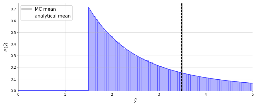
This result is not obvious to me, and I haven’t seen the equation before—hence why I’m deriving it. So to sanity check it, I used Monte Carlo sampling. In Figure $2$, I generated a normalized histogram from one million samples from the truncated lognormal distribution and compared this to its PDF. I then compared the empirical mean to the mean using Equation $15$. This suggests that we’ve derived the mean of the truncated lognormal distribution correctly.

Figure 2. Monte Carlo estimation of the lognormal distribution and its mean, compared with the mean derived in Equation $15$. The parameters used were $\mu = 0$, $\sigma = 1$, and $k = 1.5$.

Here is the Python code used to generate this figure.

from scipy.stats import norm, lognorm

N = norm(0, 1).cdf

def trunc_lognorm_pdf(xx, mu, sigma, k):
    ln_dist = lognorm(scale=np.exp(mu), s=sigma)
    numer = ln_dist.pdf(xx)
    numer[xx <= k] = 0
    denom = 1 - ln_dist.cdf(k)
    return numer / denom

def trunc_lognorm_mean(mu, sigma, k):
    z = (np.log(k) - mu) / sigma
    return np.exp(mu + 0.5 * sigma**2) * N(sigma - z) / (1 - N(z))

def trunc_lognorm_rvs(mu, sigma, k, size=1):
    out = np.empty(0)
    while out.size != size:
        xx = lognorm(scale=np.exp(mu), s=sigma).rvs(size=size)
        out = np.append(out, xx[xx > k])[:size]
    return out

See this appendix for details on SciPy’s parameterization of its lognormal implementation (lognorm).