Geometry of the Efficient Frontier

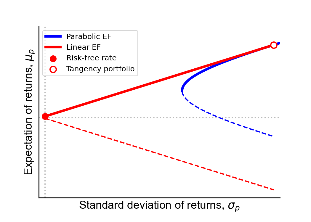
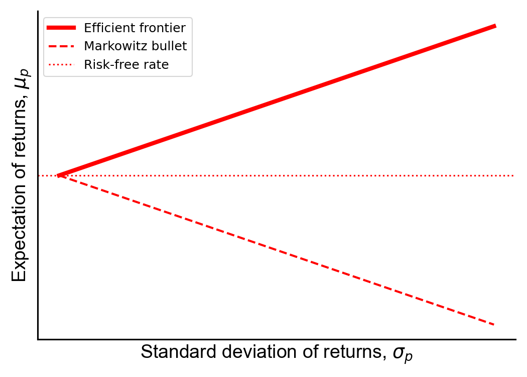
In modern portfolio theory, the efficient frontier is the locus of points $\{(\sigma_p, \mu_p)\}$ corresponding to optimal portfolios, where “optimal” means the lowest risk (standard deviation of the portfolio $\sigma_p$) for the highest reward (expected portfolio return $\mu_p$). When a portfolio contains only risky (random) assets, the relationship between risk $\sigma_p$ and reward $\mu_p$ is quadratic and is typically diagrammed as the Markowitz bullet (Figure $1$, dashed blue line) on a risk–return spectrum, with risk on the $x$-axis and reward on the $y$-axis. For any given risk $\sigma_p$, there are two portfolios on the hyperbola with different rewards. Clearly, all things being equal, higher reward should be preferred for the same level of risk. Thus, only the top half of the hyperbola is called the efficient frontier (Figure $1$, solid blue line).

This nonlinear efficient frontier only applies to portfolios with all risky assets. If we include a single risk-free asset—the canonical example is a United States treasury bill—then the Markowitz bullet becomes piecewise-linear (Figure $1$, red dashed line), and the top half is again the efficient frontier (Figure $1$, red solid line). For a given level of risk, every portfolio on this linear efficient frontier has a greater or equal expected return to any portfolio on the hyperbolic efficient frontier. The line crosses the $y$-axis at the rate of return of the risk-free asset, called the risk-free rate (Figure $1$, red circle), and the line intersects the efficient frontier at a point called the tangency portfolio (Figure $1$, white circle). The tangency portfolio gets its name because the linear efficient frontier is collinear to the tangent line at the point that the two frontiers intersect.

Finally, the slope of the linear efficient frontier is the Sharpe ratio, or the performance of a portfolio in excess of the risk-free rate after adjusting for risk. Put differently, every portfolio on the linear efficient frontier, including the tangency portfolio, has the same Sharpe ratio. Furthermore, this Sharpe ratio is the highest Sharpe possible, i.e. it is the highest expected excess return per unit risk of any portfolio.

Figure 1. The efficient frontier (EF) for risky-only assets (blue) and for a portfolio with risky and one risk-free asset (red). The inefficient frontiers are the dashed lines, since any portfolio above the axes of symmetry have higher expected return for the same risk. The linear efficient frontier is a line between the risk-free rate (red dot) and the tangency portfolio (white dot).

The above three paragraphs make a lot of claims. In many resources discussing modern portfolio theory, mean–variance analysis, or related topics such as the capital asset pricing model, these claims are often made without proof. The reader is expected to know, understand, or simply accept that everything I’ve written above makes sense. The goal of this post is to re-derive these geometric properties for myself.

These questions have already been answered in (Merton, 1972), and this post is, essentially, my notes on that paper. I’ve also relied on these notes by Eric Zivot for some of the matrix algebra required.

Setup and notation

If this section does not make sense, please see my post on mean–variance analysis first.

Suppose a portfolio has $N$ risky assets. Let $R_n$, a random variable, be the return for the $n$-th asset. Let’s denote the first moment as $\mu_n \triangleq \mathbb{E}[R_n]$, and let’s denote the covariance between $R_n$ and $R_m$ as $\sigma_{nm} \triangleq \text{Cov}(R_n, R_m)$. Thus, the variance of $R_n$ is $\sigma_{nn} = \sigma_n^2 \triangleq \mathbb{V}[R_n]$. Finally, let $w_n$ denote portfolio weight of the $n$-th asset. We can pack these symbols into vectors and a matrix as follows:

$\boldsymbol{\mu} \triangleq \begin{bmatrix} \mu_1 \\ \vdots \\ \mu_N \end{bmatrix}, \quad \boldsymbol{\Sigma} = \begin{bmatrix} \sigma_{11} & \dots & \sigma_{1N} \\ \vdots & \ddots & \vdots \\ \sigma_{N1} & \dots & \sigma_{NN} \end{bmatrix}, \quad \mathbf{w} \triangleq \begin{bmatrix} w_1 \\ \vdots \\ w_N \end{bmatrix}. \tag{1}$

We assume that the covariance matrix $\boldsymbol{\Sigma}$ is non-singular, so $\boldsymbol{\Sigma}^{-1}$ exists.

A portfolio’s return $R_p$, also a random variable, is simply an accounting identity,

$R_p \triangleq \sum_{n} w_n R_n, \tag{2}$

and we can derive it’s mean $\mu_p \triangleq \mathbb{E}[R_p]$ and variance $\sigma_p \triangleq \mathbb{V}[R_p]$ from Equation $2$:

$\begin{aligned} \mu_p &\triangleq \mathbf{w}^{\top} \boldsymbol{\mu}, \\ \sigma_p^2 &\triangleq \mathbf{w}^{\top} \boldsymbol{\Sigma} \mathbf{w}. \end{aligned} \tag{3}$

The optimal portfolio weights are defined in the following quadratic programming problem:

$\begin{aligned} \min_{\mathbf{w}} &&& \mathbf{w}^{\top} \boldsymbol{\Sigma} \mathbf{w}, \\ \text{subject to} &&& \mathbf{w}^{\top} \boldsymbol{\mu} = \mu_p, \\ \text{and} &&& \mathbf{w}^{\top} \mathbf{1} = 1, \end{aligned} \tag{4}$

In words, Equation $4$ means: minimize the portfolio’s variance subject to the constraints that the portfolio’s expected return is $\mu_p$ and the weights sum to unity. Thus, for a given expected return $\mu_p$, we can solve the optimization problem for $\mathbf{w}$ and then calculate $\sigma_p^2$.

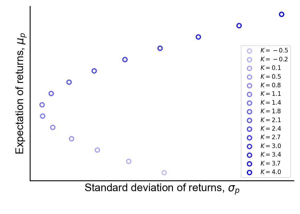
Figure 2. Fifteen portfolios on the efficient frontier, computed numerically using quadratic programming.

The Markowitz bullet is the locus of points $\{(\mu_p, \sigma_p)\}$ that satisfy Equation $4$ for all $\mu_p$, and the efficient frontier is the top half of this bullet.

In Figure $2$, I’ve drawn the Markowitz bullet for fifteen different $\mu_p$ values using synthetic expected returns $\boldsymbol{\mu}$ and covariances $\boldsymbol{\Sigma}$. For each $\mu_p$, I used SciPy’s minimize function to find the optimal weights $\mathbf{w}$ and then solved for $\sigma_p$. (See A1 for code.) Empirically, we can see that the Markowitz bullet is a hyperbola. Now, let’s prove it.

Efficient frontier with only risky assets

First, let’s derive the efficient frontier when our portfolio only contains risky assets, i.e. when each $R_n$ is a random variable. As we will see, in this case, the efficient frontier in mean-standard deviation space is a hyperbola because the portfolio variance $\sigma_p^2$ is a quadratic function of the portfolio mean $\mu_p$, i.e. the efficient frontier in mean-variance space is a parabola. We’ll prove this by solving for the optimal weights $\mathbf{w}$ using the method of Lagrange multipliers, and then expressing $\sigma_p^2$ in terms of these optimal weights.

Solving for optimal portfolio weights

Let’s write Equation $4$ using a Lagrangian function:

$\mathcal{L}(\mathbf{w}, \boldsymbol{\lambda}) = \mathbf{w}^{\top} \boldsymbol{\Sigma} \mathbf{w} + \lambda_1 \left( \mathbf{w}^{\top} \boldsymbol{\mu} - \mu_p \right) + \lambda_2 \left( \mathbf{w}^{\top} \mathbf{1} - 1 \right), \tag{5}$

where $\boldsymbol{\lambda} = \begin{bmatrix} \lambda_1 & \lambda_2 \end{bmatrix}^{\top}$ are Lagrange multipliers. We want to take the derivative of $\mathcal{L}$ w.r.t. each $w_i$ and each $\lambda_i$, set each equation equal to zero, and solve. In other words, we want to solve

$\nabla_{w_1, \dots, w_N,\lambda_1,\lambda_2} \mathcal{L}(\mathbf{w}, \boldsymbol{\lambda}) = \mathbf{0}. \tag{6}$

This is a system of $N+2$ equations. The gradient of the Lagrangian function is

$\begin{aligned} \nabla_{\mathbf{w}} \mathcal{L} &= 2 \boldsymbol{\Sigma} \mathbf{w} + \lambda_1 \boldsymbol{\mu} + \lambda_2 \mathbf{1}, \\ \frac{\partial}{\partial \lambda_1} \mathcal{L} &= \mathbf{w}^{\top} \boldsymbol{\mu} - \mu_p, \\ \frac{\partial}{\partial \lambda_2} \mathcal{L} &= \mathbf{w}^{\top} \mathbf{1} - 1. \end{aligned} \tag{7}$

The derivative of the first term in the top row of Equation $7$ is because, in general,

$\nabla_{\mathbf{x}} \; \mathbf{x}^{\top} \mathbf{B} \mathbf{x} = (\mathbf{B} + \mathbf{B}^{\top}) \mathbf{x}, \tag{8}$

for a vector $\mathbf{x}$ and matrix $\mathbf{B}$. In our case, $\mathbf{B} = \boldsymbol{\Sigma}$ is symmetric. You can easily derive this result yourself by hand or see Equation $81$ in (Petersen et al., 2008). The derivatives of the other terms are fairly straightforward.

We can solve for $\mathbf{w}$ after setting the first line of Equation $7$ to zero:

$\mathbf{w} = -\frac{1}{2} \lambda_1 \boldsymbol{\Sigma}^{-1} \boldsymbol{\mu} -\frac{1}{2} \lambda_2 \boldsymbol{\Sigma}^{-1} \mathbf{1}. \tag{9}$

This can be written more compactly as

$\begin{aligned} \mathbf{w} &= -\frac{1}{2} \boldsymbol{\Sigma}^{-1} \begin{bmatrix} \boldsymbol{\mu} & \mathbf{1} \end{bmatrix} \begin{bmatrix} \lambda_1 \\ \lambda_2 \end{bmatrix} \\ &= -\frac{1}{2} \boldsymbol{\Sigma}^{-1} \mathbf{U} \boldsymbol{\lambda}. \end{aligned} \tag{10}$

where $\mathbf{U}$ is an $N \times 2$ matrix, $\mathbf{U} \triangleq \begin{bmatrix} \boldsymbol{\mu} & \mathbf{1} \end{bmatrix}$.

We can solve for $\boldsymbol{\lambda}$ while adhering to the equation for $\mathbf{w}$ by plugging Equation $10$ into the second and third lines of Equation $7$ after setting these lines equal to zero:

$\begin{aligned} \mu_p = \boldsymbol{\mu}^{\top} \mathbf{w} &= -\frac{1}{2} \lambda_1 \boldsymbol{\mu}^{\top} \boldsymbol{\Sigma}^{-1} \boldsymbol{\mu} -\frac{1}{2} \lambda_2 \boldsymbol{\mu}^{\top} \boldsymbol{\Sigma}^{-1} \mathbf{1}, \\ 1 = \mathbf{1}^{\top} \mathbf{w} &= -\frac{1}{2} \lambda_1 \mathbf{1}^{\top} \boldsymbol{\Sigma}^{-1} \boldsymbol{\mu} -\frac{1}{2} \lambda_2 \mathbf{1}^{\top} \boldsymbol{\Sigma}^{-1} \mathbf{1}. \end{aligned} \tag{11}$

We can write this system of linear equations in matrix form as

$\begin{aligned} \begin{bmatrix} \mu_p \\ 1 \end{bmatrix} &= -\frac{1}{2} \begin{bmatrix} \boldsymbol{\mu}^{\top} \boldsymbol{\Sigma}^{-1} \boldsymbol{\mu} & \boldsymbol{\mu}^{\top} \boldsymbol{\Sigma}^{-1} \mathbf{1} \\ \mathbf{1}^{\top} \boldsymbol{\Sigma}^{-1} \boldsymbol{\mu} & \mathbf{1}^{\top} \boldsymbol{\Sigma}^{-1} \mathbf{1} \end{bmatrix} \begin{bmatrix} \lambda_1 \\ \lambda_2 \end{bmatrix} \\ &= -\frac{1}{2} \begin{bmatrix} \boldsymbol{\mu}^{\top} \\ \mathbf{1}^{\top} \end{bmatrix} \boldsymbol{\Sigma}^{-1} \begin{bmatrix} \boldsymbol{\mu} & \mathbf{1} \end{bmatrix} \boldsymbol{\lambda}. \end{aligned} \tag{12}$

We can simplify Equation $12$ by writing it in terms of $\mathbf{U}$, $\boldsymbol{\lambda}$, $\mathbf{u} \triangleq \begin{bmatrix} \mu_p & 1 \end{bmatrix}^{\top}$, and $\mathbf{M} \triangleq \mathbf{U}^{\top} \boldsymbol{\Sigma}^{-1} \mathbf{U}$:

$\begin{aligned} \mathbf{u} &= -\frac{1}{2} \mathbf{U}^{\top} \boldsymbol{\Sigma}^{-1} \mathbf{U} \boldsymbol{\lambda} \\ &= -\frac{1}{2} \mathbf{M} \boldsymbol{\lambda}. \end{aligned} \tag{13}$

Now we can solve for the $\boldsymbol{\lambda}$ values which hold for Equation $10$:

$\boldsymbol{\lambda} = -2 \mathbf{M}^{-1} \mathbf{u}. \tag{14}$

And finally, we can solve explicitly for the optimal weights that give the efficient frontier $\mathbf{w}$ by plugging Equation $14$ into the second line of Equation $10$:

$\mathbf{w}^{\star} = \boldsymbol{\Sigma}^{-1} \mathbf{U} \mathbf{M}^{-1} \mathbf{u}. \tag{15}$

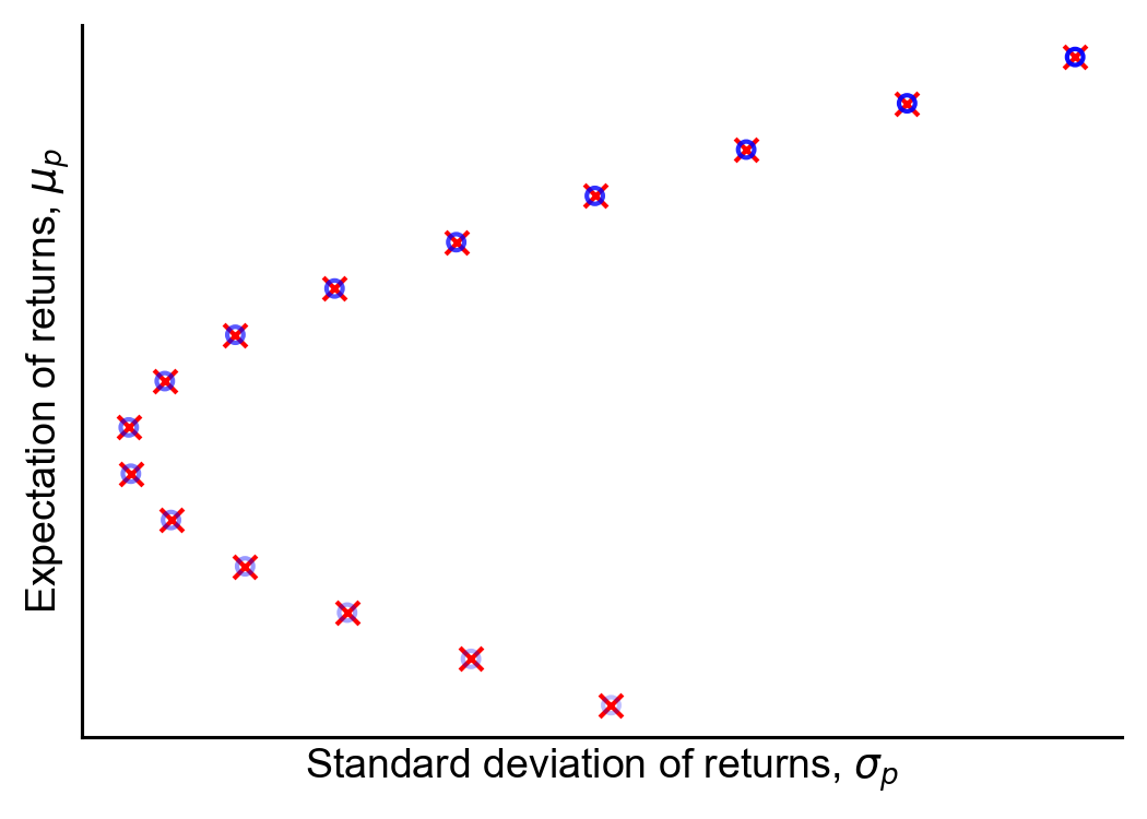
To check that this is correct, I’ve re-created Figure $2$ using both numerical minimization of Equation $4$ and analytical computation of Equation $15$ (Figure $3$). (See A2 for code.)

Figure 3. Fifteen portfolios on the efficient frontier, computed numerically using quadratic programming (blue dots) and analytically using Equation $15$ (red "x" marks).

Why the Markowitz bullet is a hyperbola

So why is the Markowitz bullet a hyperbola? We can now express the portfolio variance $\sigma_p^2$ as a function of its expected return $\mu_p$ (encoded in $\mathbf{u}$):

$\begin{aligned} \sigma_p^2 &= \mathbf{w}^{\top} \boldsymbol{\Sigma} \mathbf{w} \\ &= (\boldsymbol{\Sigma}^{-1} \mathbf{U} \mathbf{M}^{-1} \mathbf{u})^{\top} \boldsymbol{\Sigma} (\boldsymbol{\Sigma}^{-1} \mathbf{U} \mathbf{M}^{-1} \mathbf{u}) \\ &= \mathbf{u}^{\top} \mathbf{M}^{-1} \mathbf{U}^{\top} \boldsymbol{\Sigma}^{-1} \mathbf{U} \mathbf{M}^{-1} \mathbf{u}. \\ &= \mathbf{u}^{\top} \mathbf{M}^{-1} \mathbf{u}. \\ &= \begin{bmatrix} \mu_p & 1 \end{bmatrix} \left[ \begin{bmatrix} \boldsymbol{\mu}^{\top} \\ \mathbf{1}^{\top} \end{bmatrix} \boldsymbol{\Sigma}^{-1} \begin{bmatrix} \boldsymbol{\mu} & \mathbf{1} \end{bmatrix} \right]^{-1} \begin{bmatrix} \mu_p \\ 1 \end{bmatrix} \end{aligned} \tag{16}$

At this point, we need to invert $\mathbf{M}$, but it’s not as bad as it looks because $\mathbf{M}$ is a $2 \times 2$ matrix:

$\mathbf{M} = \begin{bmatrix} \boldsymbol{\mu}^{\top} \\ \mathbf{1}^{\top} \end{bmatrix} \boldsymbol{\Sigma}^{-1} \begin{bmatrix} \boldsymbol{\mu} & \mathbf{1} \end{bmatrix} = \begin{bmatrix} \boldsymbol{\mu}^{\top} \boldsymbol{\Sigma}^{-1} \boldsymbol{\mu} & \boldsymbol{\mu}^{\top} \boldsymbol{\Sigma}^{-1} \mathbf{1} \\ \mathbf{1}^{\top} \boldsymbol{\Sigma}^{-1} \boldsymbol{\mu} & \mathbf{1}^{\top} \boldsymbol{\Sigma}^{-1} \end{bmatrix}. \tag{17}$

Recall that the inverse of a $2 \times 2$ matrix $\mathbf{A}$ has the following solution:

$\mathbf{A} = \begin{bmatrix} a & b \\ c & d \end{bmatrix}, \qquad \mathbf{A}^{-1} = \frac{1}{\det(\mathbf{A})} \begin{bmatrix} d & -b \\ -c & a \end{bmatrix}, \qquad \det(\mathbf{A}) = ad - bc. \tag{18}$

This is particularly convenient for us since $\mathbf{M}$ is symmetric. Therefore, the inverse of $\mathbf{M}$ is just

$\mathbf{M}^{-1} = \frac{1}{\det(\mathbf{M})} \begin{bmatrix} \mathbf{1}^{\top} \boldsymbol{\Sigma}^{-1} \mathbf{1} & -\mathbf{1}^{\top} \boldsymbol{\Sigma}^{-1} \boldsymbol{\mu} \\ -\boldsymbol{\mu}^{\top} \boldsymbol{\Sigma}^{-1} \mathbf{1} & \boldsymbol{\mu}^{\top} \boldsymbol{\Sigma}^{-1} \boldsymbol{\mu} \end{bmatrix}. \tag{19}$

Putting it all together, we can see that the variance of the portfolio $\sigma_p^2$ is a quadratic function of its expected return $\mu_p$:

$\sigma_p^2 = \frac{1}{\det(\mathbf{M})} \left\{ (\mathbf{1}^{\top} \boldsymbol{\Sigma}^{-1} \mathbf{1}) \mu_p^2 - 2 (\mathbf{1}^{\top} \boldsymbol{\Sigma}^{-1} \boldsymbol{\mu}) \mu_p + \boldsymbol{\mu}^{\top} \boldsymbol{\Sigma}^{-1} \boldsymbol{\mu} \right\}. \tag{20}$

This is just a vectorized formulation of Equation $12$ in (Merton, 1972). To quote Merton on his Equation $12$, “Thus, the frontier in mean-variance space is a parabola.” Later, we will find it easier to work with this quadratic equation if we introduce some notation:

$\begin{aligned} s_{11} &\triangleq \mathbf{1}^{\top} \boldsymbol{\Sigma}^{-1} \mathbf{1}, \\ s_{1\mu} = s_{\mu 1} &\triangleq \mathbf{1}^{\top} \boldsymbol{\Sigma}^{-1} \boldsymbol{\mu}, \\ s_{\mu\mu} &\triangleq \boldsymbol{\mu}^{\top} \boldsymbol{\Sigma}^{-1} \boldsymbol{\mu} \\ d &\triangleq \det(\mathbf{M}) = s_{\mu\mu}s_{11} - s_{1\mu}^2. \end{aligned} \tag{21}$

Putting it together, we can write $\mu_p$ in terms of $\sigma_p$ as

$\sigma_p = f(\mu_p) = \sqrt{\frac{s_{11} \mu_p^2 - 2 s_{1\mu} \mu_p + s_{\mu\mu}}{d}}. \tag{22}$

And this is just a vectorized formulation of Equation $15$ in (Merton, 1972). To quote Merton again, “It is usual to present the frontier in the mean-standard deviation plane instead of the mean-variance plane… Figure II graphs [this] frontier which is a hyperbola…” To summarize, the efficient frontier in terms of $(\mu_p, \sigma_p^2)$ is a parabola, while the efficient frontier in terms of $(\mu_p, \sigma_p)$ is a hyperbola. And “Markowitz bullet” typically refers to the frontier in mean-standard deviation space, i.e. the bullet is a hyperbola. This is a subtle distinction which was pointed out to me by a reader (see the acknowledgements). See this mathematics StackExchange post for further discussion.

Anyway, Equation $22$ is useful is because now we can use basic properties of quadratic equations for quick computation, such as finding the vertex of the hyperbola (where the efficient frontier starts), taking derivatives, or solving for $\mu_p$.

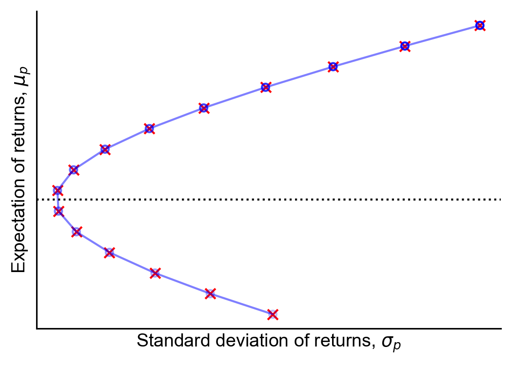
Figure 4. The Markowitz bullet (blue line), visualized by drawing ten thousand portfolios that satisfy Equation $20$. Also, fifteen portfolios on the efficient frontier, computed numerically using quadratic programming (blue dots) and analytically using Equation $15$ (red "x" marks).

Furthermore, we can easily vectorize the computation required to draw the efficient frontier. Rather than computing the optimal $\mathbf{w}$ and then computing $\sigma_p^2$, we can simply compute the three scalar coefficients in Equation $22$—which do not depend on $\mathbf{w}$—and the normalization term $d$ to compute the correct (minimum) standard deviation $\sigma_p$ for any input expected return $\mu_p$. In Figure $4$, I have drawn the Markowitz bullet using this vectorized computation over ten thousand $\mu_p$ values. (See A3 for code.)

Relationship between reward and weights

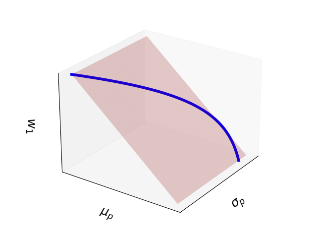
Finally, note that Equation $15$ has an important implication. While the relationship between risk and reward is quadratic, the relationship between optimal weights and expected returns is linear. Thus, the Markowitz bullet is just hyperplane in weight-space. To visualize this, I’ve plotted the Markowitz bullet for $N=2$ assets. When $N=2$, the two optimal weights are fully specified by $w_1$, since $w_2 = 1 - w_1$. Thus, we can plot the Markowitz bullet in $3$-dimensional space, with $\sigma_p$, $\mu_p$, and $w_1$ as the axes (Figure $5$).

Figure 5. The Markowitz bullet in $3$-dimensional space defined by expected return $\mu_p$, return variance $\sigma_p$, and optimal weight $w_1$. The bullet is a hyperbola lying on a hyperplane defined by $w_1$.

Intuitively, this makes sense. All this geometry is representing is that, if we want bigger expected returns for our portfolio, we should put more weight on assets with bigger expected returns. However, our risk grows nonlinearly.

Efficient frontier with a risk-less asset

Now that we have proven that the Markowitz bullet with risky assets is a hyperbola, let’s consider the efficient frontier when we include a risk-free asset with return $r_f$ (lowercase because non-random). As I mentioned, this is often called the risk-free rate and the canonical example of a risk-free asset is a United States treasury bill. We’ll prove that, in this case, the Markowitz bullet is a piecewise linear function, and that the slope of the top half of this frontier—the efficient part—is the Sharpe ratio. Where the hyperbolic and linear functions intersect is called the tangency portfolio (Figure $1$).

Note that we will assume the risk-free rate $r_f$ is lower than the $y$-coordinate of the vertex of the hyperbolic efficient frontier. In other words, we assume that a portfolio of risky assets has higher expected return than the risk-free rate. See Section IV of (Merton, 1972) for a discussion of when this does not hold.

To compute this new efficient frontier, let’s repeat our process from the previous section, but this time, let’s include a risk-free asset. Let $w_f$ denote the weight of $r_f$ in a portfolio with $N+1$ assets. Since the portfolio weights sum to unity, we have

$\mathbf{w}^{\top} \mathbf{1} + w_f = 1. \tag{23}$

The expected return on a portfolio with both risky and risk-free assets can be written as

$\begin{aligned} \mu_p &= \mathbf{w}^{\top} \boldsymbol{\mu} + w_f r_f \\ &= \mathbf{w}^{\top} \boldsymbol{\mu} + r_f (1 - \mathbf{w}^{\top} \mathbf{1}) \\ &= r_f + \mathbf{w}^{\top} (\boldsymbol{\mu} - r_f \mathbf{1}). \end{aligned} \tag{24}$

Since $r_f$ is risk-free, we want to minimize our portfolio’s variance, which is still $\mathbf{w}^{\top} \boldsymbol{\Sigma} \mathbf{w}$, while targeting a given expected excess return, which is just the expected return less the risk-free rate,

$\mu_p - r_f = \mathbf{w}^{\top} (\boldsymbol{\mu} - r_f \mathbf{1}). \tag{25}$

We target the excess return because $r_f$ is fixed. To simplify things, let’s use the following notation:

$\begin{aligned} \tilde{\boldsymbol{\mu}} &\triangleq \boldsymbol{\mu} - r_f \mathbf{1}, \\ \tilde{\mu}_p &\triangleq \mu_p - r_f. \end{aligned} \tag{26}$

Now the new optimization problem is

$\begin{aligned} \min_{\mathbf{w}} &&& \mathbf{w}^{\top} \boldsymbol{\Sigma} \mathbf{w}, \\ \text{subject to} &&& \mathbf{w}^{\top} \tilde{\boldsymbol{\mu}} = \tilde{\mu}_p. \end{aligned} \tag{27}$

Notice that $\mathbf{w}^{\top} \mathbf{1} = 1$ is no longer a constraint. While the portfolio weights must sum to unity, $\mathbf{w}$ need not. This is because we can allocate whatever proportion of our portfolio we would like to the risk-free asset. The portfolio variance is unchanged since $r_f$ is risk-free. Again, we can solve this using Lagrange multipliers. The Lagrangian is

$\mathcal{L}(\mathbf{w}, \lambda) = \mathbf{w}^{\top} \boldsymbol{\Sigma} \mathbf{w} + \lambda (\mathbf{w}^{\top} \tilde{\boldsymbol{\mu}} - \tilde{\mu}_p). \tag{28}$

Again, we can find the first-order conditions by computing the gradient, setting it equal to zero, and following for $\mathbf{w}$ in terms of $\lambda$. The first-order conditions are

$\begin{aligned} \nabla_{\mathbf{w}} \mathcal{L} &= 2 \boldsymbol{\Sigma} \mathbf{w} + \lambda \tilde{\boldsymbol{\mu}} = \mathbf{0}, \\ \frac{\partial}{\partial \lambda} \mathcal{L} &= \mathbf{w}^{\top} \tilde{\boldsymbol{\mu}} - \tilde{\mu}_p = 0. \end{aligned} \tag{29}$

As before, let’s solve the first first-order condition for $\mathbf{w}$:

$\mathbf{w} = -\frac{\lambda}{2} \boldsymbol{\Sigma}^{-1} \tilde{\boldsymbol{\mu}}. \tag{30}$

We can then solve for $\lambda$ while adhering to the definition of $\mathbf{w}$ as before:

$\begin{aligned} \tilde{\mu}_p &= \tilde{\boldsymbol{\mu}}^{\top} \mathbf{w} \\ &= -\frac{\lambda}{2} \tilde{\boldsymbol{\mu}}^{\top} \boldsymbol{\Sigma}^{-1} \tilde{\boldsymbol{\mu}}, \\ &\Downarrow \\ \lambda &= \frac{-2 \tilde{\mu}_p}{\tilde{\boldsymbol{\mu}}^{\top} \boldsymbol{\Sigma}^{-1} \tilde{\boldsymbol{\mu}}}. \end{aligned} \tag{31}$

Finally, we can plug $\lambda$ back into Equation $30$ to solve for $\mathbf{w}$ without $\lambda$:

$\mathbf{w} = \tilde{\mu}_p \left( \frac{\boldsymbol{\Sigma}^{-1} \tilde{\boldsymbol{\mu}}}{\tilde{\boldsymbol{\mu}}^{\top} \boldsymbol{\Sigma}^{-1} \tilde{\boldsymbol{\mu}}} \right). \tag{32}$

(This is Merton’s Equation $36$.) As before, we can now express $\sigma_p^2$ in terms of these optimal weights:

$\begin{aligned} \sigma_p^2 &= \mathbf{w}^{\top} \boldsymbol{\Sigma} \mathbf{w} \\ &= \tilde{\mu}_p^2 \left( \frac{\boldsymbol{\Sigma}^{-1} \tilde{\boldsymbol{\mu}}}{\tilde{\boldsymbol{\mu}}^{\top} \boldsymbol{\Sigma}^{-1} \tilde{\boldsymbol{\mu}}} \right)^{\top} \boldsymbol{\Sigma} \left( \frac{\boldsymbol{\Sigma}^{-1} \tilde{\boldsymbol{\mu}}}{\tilde{\boldsymbol{\mu}}^{\top} \boldsymbol{\Sigma}^{-1} \tilde{\boldsymbol{\mu}}} \right) \\ &= \frac{(\mu_p - r_f)^2}{(\boldsymbol{\mu} - r_f \mathbf{1})^{\top} \boldsymbol{\Sigma}^{-1} (\boldsymbol{\mu} - r_f \mathbf{1})}. \end{aligned} \tag{33}$

This time, rather than leaving this as a function of $\mu_p$, let’s rewrite it as a function of $\sigma_p$, so that we can easily plot it the standard mean–variance axes:

$\begin{aligned} | \mu_p - r_f | &= \sigma_p \sqrt{(\boldsymbol{\mu} - r_f \mathbf{1})^{\top} \boldsymbol{\Sigma}^{-1} (\boldsymbol{\mu} - r_f \mathbf{1})} \\ &\Downarrow \\ \mu_p &= r_f \pm \sigma_p \sqrt{(\boldsymbol{\mu} - r_f \mathbf{1})^{\top} \boldsymbol{\Sigma}^{-1} (\boldsymbol{\mu} - r_f \mathbf{1})}. \end{aligned} \tag{34}$

Note that this is Merton’s Equation $35$. Clearly, the Markowitz bullet is now a piecewise linear function, and again, the efficient frontier is only the top-half of this bullet (Figure $6$).

Figure 6. The Markowitz bullet is a piecewise linear function when a portfolio can contain one risk-less asset. The efficient frontier is the top half of this bullet, a line. The vertex is the risk-free rate.

Notice that the slope of this new frontier with a risk-less asset is the Sharpe ratio:

$\frac{\mu_p - r_f}{\sigma_p} = \sqrt{(\boldsymbol{\mu} - r_f \mathbf{1})^{\top} \boldsymbol{\Sigma}^{-1} (\boldsymbol{\mu} - r_f \mathbf{1})}. \tag{35}$

Thus, we have a geometric interpretation of the Sharpe ratio: it is reward (expected excess return) per unit risk (standard deviation) on the risk–return spectrum. A higher Sharpe is a steeper slope, meaning more reward for the same risk. The right-hand side of Equation $35$ is just the Sharpe ratio of any portfolio along the linear efficient frontier.

Sharpe-maximizing portfolio

So all portfolios on the linear efficient frontier have the same Sharpe (Equation $35$). A natural question to ask at this point is: since portfolios on the hyperbolic efficient frontier have varying Sharpe ratios, which one has maximum Sharpe?

To find this portfolio, we just need to compute

$\mu_p^{\textsf{max}} = \arg\!\max_{x} \left\{ \frac{x - r_f}{\sigma_p^{\textsf{min}}} \right\}, \tag{36}$

where $\sigma_p^{\textsf{min}}$ is the minimum variance (Equation $22$). We can drop the determinant since it does not depend on $x$, giving us the following optimization problem:

$\mu_p^{\textsf{max}} = \arg\!\max_{x} \left\{ \frac{x - r_f}{\sqrt{s_{11} x^2 - 2 s_{1\mu} x + s_{\mu\mu}}} \right\}. \tag{37}$

Again, we take the derivative, set it equal to zero, and solve for $x$. The first-order condition is:

$\frac{\partial}{\partial x} \left[ (x - r_f) (s_{11} x^2 - 2 s_{1\mu} x + s_{\mu\mu})^{-1/2} \right] = 0. \tag{38}$

Using the product rule, we get:

$(s_{11} x^2 - 2 s_{1\mu} x + s_{\mu\mu})^{-1/2} - \frac{1}{2} \frac{(2 s_{11} x - 2 s_{1\mu}) (x - r_f)}{(s_{11} x^2 - 2 s_{1\mu} x + s_{\mu\mu})^{3/2}} = 0. \tag{39}$

We can eliminate the $n$-roots by multiplying both sides of the equation by the denominator in the rightmost term in Equation $39$ and then simplifying:

$\begin{aligned} 0 &= (s_{11} x^2 - 2 s_{1\mu} x + s_{\mu\mu}) - (s_{11} x - s_{1\mu})(x-r_f) \\ 0 &= s_{11} x^2 - 2 s_{1\mu} x + s_{\mu\mu} - (s_{11} x^2 - s_{1\mu} x - s_{11} r_f x + s_{1\mu} r_f) \\ 0 &= \cancel{s_{11} x^2} - 2 s_{1\mu} x + s_{\mu\mu} - \cancel{s_{11} x^2} + s_{1\mu} x + s_{11} r_f x - s_{1\mu} r_f \\ -s_{1\mu} x + s_{11} r_f x &= -s_{\mu\mu} + s_{1\mu} r_f \\ x &= \frac{-s_{\mu\mu} + s_{1\mu} r_f}{-s_{1\mu} + s_{11} r_f}. \end{aligned} \tag{40}$

Thus, we have shown that the optimal portfolio weights are:

$\mu_p^{\textsf{max}} = \frac{s_{\mu\mu} - r_f s_{1\mu}}{s_{1\mu} - r_f s_{11}}. \tag{41}$

Let’s plug this into Equation $15$, since these are the optimal weights for a portfolio on the quadratic efficient frontier. The only place that $\mu_p^{\textsf{max}}$ appears is in $\mathbf{u}$. Let’s compute just $\mathbf{M}^{-1} \mathbf{u}$ first, since it is tedious. To be clear, we want to compute

$\mathbf{M}^{-1} \mathbf{u} = \frac{1}{d} \begin{bmatrix} s_{11} & -s_{1\mu} \\ -s_{1\mu} & s_{\mu\mu} \end{bmatrix} \begin{bmatrix} \frac{s_{\mu\mu} - r_f s_{1\mu}}{s_{1\mu} - r_f s_{11}} \\ 1 \end{bmatrix}. \tag{42}$

Let’s compute each component in the resultant $2$-vector separately. The first component is

$\begin{aligned} & \frac{1}{d} \left[ s_{11} \left( \frac{s_{\mu\mu} - r_f s_{1\mu}}{s_{1\mu} - r_f s_{11}} \right) - s_{1\mu} \right] \\ &= \frac{1}{d} \left[ \frac{s_{11} s_{\mu\mu} - r_f s_{11} s_{1\mu} - s_{1\mu}^2 + r_f s_{11} s_{1\mu}}{s_{1\mu} - r_f s_{11}} \right] \\ &= \frac{1}{d} \left[ \frac{s_{11} s_{\mu\mu} - s_{1\mu}^2}{s_{1\mu} - r_f s_{11}} \right] \\ &= \frac{1}{s_{1\mu} - r_f s_{11}}. \end{aligned} \tag{43}$

The second component is

$\begin{aligned} & \frac{1}{d} \left[ -s_{1\mu} \left( \frac{s_{\mu\mu} - r_f s_{1\mu}}{s_{1\mu} - r_f s_{11}} \right) - s_{\mu\mu} \right] \\ &= \frac{1}{d} \left[ \frac{-s_{1\mu} s_{\mu\mu} + r_f s_{1\mu}^2 + s_{\mu\mu} s_{1\mu} - r_f s_{11} s_{\mu\mu}}{s_{1\mu} - r_f s_{11}} \right] \\ &= \frac{1}{d} \left[ \frac{r_f s_{1\mu}^2 - r_f s_{11} s_{\mu\mu}}{s_{1\mu} - r_f s_{11}} \right] \\ &= \frac{1}{d} \left[ \frac{-r_f (s_{11} s_{\mu\mu} - s_{1\mu}^2)}{s_{1\mu} - r_f s_{11}} \right] \\ &= \frac{-r_f}{s_{1\mu} - r_f s_{11}}. \end{aligned} \tag{44}$

Now putting these two rows into a vector and right-multiplying it by $\boldsymbol{\Sigma}^{-1} \mathbf{U}$, we get

$\begin{aligned} \mathbf{w} &= \boldsymbol{\Sigma}^{-1} \mathbf{U} \mathbf{M}^{-1} \mathbf{u} \\ &= \begin{bmatrix} \boldsymbol{\Sigma}^{-1} \boldsymbol{\mu} & \boldsymbol{\Sigma}^{-1} \mathbf{1} \end{bmatrix} \begin{bmatrix} \frac{1}{s_{1\mu} - r_f s_{11}} \\ \frac{-r_f}{s_{1\mu} - r_f s_{11}} \end{bmatrix} \\ &= \frac{\boldsymbol{\Sigma}^{-1} \boldsymbol{\mu}}{s_{1\mu} - r_f s_{11}} - \frac{r_f \boldsymbol{\Sigma}^{-1} \mathbf{1}}{s_{1\mu} - r_f s_{11}} \\ &= \frac{\boldsymbol{\Sigma}^{-1} (\boldsymbol{\mu} - r_f \mathbf{1})}{\mathbf{1}^{\top} \boldsymbol{\Sigma}^{-1} \boldsymbol{\mu} - r_f \mathbf{1}^{\top} \boldsymbol{\Sigma}^{-1} \mathbf{1}} \\ &= \frac{\boldsymbol{\Sigma}^{-1} (\boldsymbol{\mu} - r_f \mathbf{1})}{\mathbf{1}^{\top} \boldsymbol{\Sigma}^{-1} (\boldsymbol{\mu} - r_f \mathbf{1})}. \end{aligned} \tag{45}$

Thus, the portfolio weights which maximizes the Sharpe ratio on the hyperbolic efficient frontier are

$\mathbf{w}^{\textsf{max}} \triangleq \frac{\boldsymbol{\Sigma}^{-1} (\boldsymbol{\mu} - r_f \mathbf{1})}{\mathbf{1}^{\top} \boldsymbol{\Sigma}^{-1} (\boldsymbol{\mu} - r_f \mathbf{1})}. \tag{46}$

Tangency portfolio

Now let’s derive the weights of the portfolio that sits at the intersection of hyperbolic and linear efficient frontiers. This is called the tangency portfolio, and we’ll see why in the next section. The point for this section is that the tangency portfolio has the same weights as in Equation $46$, i.e. the tangency portfolio maximizes the Sharpe ratio.

By definition, the tangency portfolio is fully invested in risky assets and has no stake in $r_f$. But since it has the weight $w_f$, it must sit at the intersection of the hyperbolic and linear efficient frontiers. Let $\boldsymbol{\omega}$ denote this $(N+1)$-vector of weights:

$\boldsymbol{\omega} = \begin{bmatrix} \mathbf{w} \\ w_f \end{bmatrix}. \tag{47}$

So while $\boldsymbol{\omega}^{\top} \mathbf{1} = 1$, we know that $w_f = 0$. Thus, we can use the result from Equation $32$ to write:

$1 = \mathbf{1}^{\top} \boldsymbol{\omega} = \mathbf{1}^{\top} \mathbf{w} = \tilde{\mu}_p \left( \frac{\mathbf{1} \boldsymbol{\Sigma}^{-1} \tilde{\boldsymbol{\mu}}}{\tilde{\boldsymbol{\mu}}^{\top} \boldsymbol{\Sigma}^{-1} \tilde{\boldsymbol{\mu}}} \right), \tag{48}$

which implies

$\tilde{\mu}_p = \frac{\tilde{\boldsymbol{\mu}}^{\top} \boldsymbol{\Sigma}^{-1} \tilde{\boldsymbol{\mu}}}{\mathbf{1} \boldsymbol{\Sigma}^{-1} \tilde{\boldsymbol{\mu}}}. \tag{49}$

Equation $49$ is a closed-form solution for the expected excess return of the tangency portfolio. And we can plug this excess return back into our equation for the portfolio weights (again Equation $32$) to get

$\begin{aligned} \mathbf{w}^{\textsf{tp}} &= \left( \frac{\tilde{\boldsymbol{\mu}}^{\top} \boldsymbol{\Sigma}^{-1} \tilde{\boldsymbol{\mu}}}{\mathbf{1} \boldsymbol{\Sigma}^{-1} \tilde{\boldsymbol{\mu}}} \right) \left( \frac{\boldsymbol{\Sigma}^{-1} \tilde{\boldsymbol{\mu}}}{\tilde{\boldsymbol{\mu}}^{\top} \boldsymbol{\Sigma}^{-1} \tilde{\boldsymbol{\mu}}} \right) \\ &= \frac{\boldsymbol{\Sigma}^{-1} \tilde{\boldsymbol{\mu}}}{\mathbf{1} \boldsymbol{\Sigma}^{-1} \tilde{\boldsymbol{\mu}}} \\ &= \frac{\boldsymbol{\Sigma}^{-1} (\boldsymbol{\mu} - r_f \mathbf{1})}{\mathbf{1} \boldsymbol{\Sigma}^{-1} (\boldsymbol{\mu} - r_f \mathbf{1})} \\ &= \mathbf{w}^{\textsf{max}} \end{aligned} \tag{50}$

Here, I’ve written $\mathbf{w}^{\textsf{tp}}$ to emphasize that this derivation only holds if we assume $w_f = 0$, i.e. that these weights are the tangency portfolio. And we see that these weights $\mathbf{w}^{\textsf{tp}}$ are equal to the weights $\mathbf{w}^{\textsf{max}}$ for the Sharpe-maximizing portfolio.

Tangent line at tangency portfolio

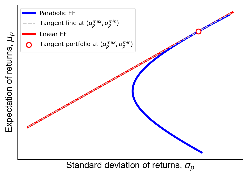
Finally, let’s see why the tangency portfolio has the name it does. We will compute the tangent line at the tangency portfolio and show that its slope is equal to the slope of the linear efficient frontier (Figure $7$). This will prove that the two lines (the linear EF and the tangent line at the tangency portfolio) are collinear, since we already know that the tangency portfolio is on the linear efficient frontier.

Figure 7. The tangent line at the tangency portfolio $(\mu_p^{\textsf{max}}, \sigma_p^{\textsf{min}})$ has a slope equal to the slope of the linear efficient frontier (EF). This point is the intersection of the hyperbolic and efficient frontiers.

Let’s see that the slope of the tangent line at $(\mu_p^{\textsf{max}}, \sigma_p^{\textsf{min}})$ is indeed Equation $35$. To find the slope of the tangent line of a function

$y = f(x) + b \tag{51}$

at a point $(x_1, y_1)$, we need to compute the derivative at $x_1$, i.e. compute $f^{\prime}(x_1)$.

The derivative of Equation $23$ is

$f^{\prime}(\mu) = \frac{s_{11} \mu - s_{1\mu}}{\sqrt{d (s_{11} \mu^2 - 2 s_{1\mu} \mu + s_{\mu\mu})}}. \tag{52}$

To find the slope of the tangent line at the tangency portfolio, we simply plug in $\mu_p^{\textsf{max}}$. For simplicity, since the derivations are tedious, let’s call this optimal value $x$. Then we have

$f^{\prime}(x) = \frac{s_{11} x - s_{1\mu}}{\sqrt{d (s_{11} x^2 - 2 s_{1\mu} x + s_{\mu\mu})}}. \tag{53}$

The numerator is

$\begin{aligned} s_{11} \left( \frac{s_{\mu\mu} - rs_{1\mu}}{s_{1\mu} - rs_{11}} \right) - s_{1\mu} \left( \frac{s_{1\mu} - rs_{11}}{s_{1\mu} - rs_{11}} \right) &= \frac{s_{11}s_{\mu\mu} - rs_{1\mu}s_{11} - s_{1\mu}^2 + rs_{1\mu}s_{11}}{s_{1\mu} - rs_{11}} \\ &= \frac{s_{11}s_{\mu\mu} - s_{1\mu}^2}{s_{1\mu} - rs_{11}} \\ &= \frac{d}{s_{1\mu} - rs_{11}}. \end{aligned} \tag{54}$

Now let’s compute the quadratic term in the denominator of Equation $53$. This is

$\begin{aligned} & s_{11}x^2 - 2s_{1\mu}x + s_{\mu\mu} \\ &= s_{11} \left( \frac{s_{\mu\mu} - rs_{1\mu}}{s_{1\mu} - rs_{11}} \right)^2 - 2s_{1\mu} \left( \frac{s_{\mu\mu} - rs_{1\mu}}{s_{1\mu} - rs_{11}} \right) + s_{\mu\mu} \\ &= \frac{s_{11} (s_{\mu\mu} - rs_{1\mu})^2 - 2s_{1\mu}(s_{\mu\mu} - rs_{1\mu})(s_{1\mu}-r s_{11}) + s_{\mu\mu}(s_{1\mu} - rs_{11})^2}{(s_{1\mu} - rs_{11})^2}. \end{aligned} \tag{55}$

We can see here that the denominator in Equation $54$ will cancel with the denominator in Equation $55$. So we only need to simplify the numerator in Equation $55$. This is

$\begin{aligned} & s_{11}(s_{\mu\mu}^2 - 2 s_{1\mu}s_{\mu\mu}r + s_{1\mu}^2 r^2) \\ &\quad - 2s_{1\mu}(s_{1\mu}s_{\mu\mu} - s_{1\mu}^2 r - s_{\mu\mu}s_{11}r + s_{1\mu}s_{11}r^2) \\ &\quad + s_{\mu\mu}(s_{1\mu}^2 - 2s_{1\mu}s_{11}r + s_{11}^2 r^2) \end{aligned} \tag{56}$

Let’s simplify by distributing, canceling, and combining like terms:

$\begin{aligned} & s_{11}s_{\mu\mu}^2 - \cancel{2s_{1\mu}s_{\mu\mu}s_{11}r} + \underline{s_{1\mu}^2s_{11}r^2} \\ &\quad - \boxed{2s_{1\mu}^2s_{\mu\mu}} + 2s_{1\mu}^3r + \cancel{2s_{1\mu}s_{\mu\mu}s_{11}r} - \underline{2s_{1\mu}^2s_{11}r^2}) \\ &\quad + \boxed{s_{1\mu}^2s_{\mu\mu}} - 2s_{1\mu}s_{\mu\mu}s_{11}r + s_{\mu\mu}s_{11}^2r^2. \end{aligned} \tag{57}$

Simplifying further, we get

$\begin{aligned} & s_{11}s_{\mu\mu}^2 - s_{1\mu}^2s_{11}r^2 - s_{1\mu}^2s_{\mu\mu} + 2s_{1\mu}^3r - 2s_{1\mu}s_{\mu\mu}s_{11}r + s_{\mu\mu}s_{11}^2r^2 \\ &= (s_{\mu\mu}s_{11}^2 - s_{1\mu}^2s_{11}) r^2 - 2(s_{1\mu}s_{\mu\mu}s_{11} - s_{1\mu}^3)r + (s_{11}s_{\mu\mu}^2 - s_{1\mu}^2s_{\mu\mu}) \\ &= s_{11} (s_{\mu\mu}s_{11} - s_{1\mu}^2) r^2 - 2 s_{1\mu}(s_{\mu\mu}s_{11} - s_{1\mu}^2)r + s_{\mu\mu} (s_{11}s_{\mu\mu} - s_{1\mu}^2) \\ &= d (s_{11} r^2 - 2 s_{1\mu} r + s_{\mu\mu}). \end{aligned} \tag{58}$

We can see that things should start canceling, giving us

$\begin{aligned} \frac{\partial \sigma}{\partial \mu} \bigg|_{\mu = x} &= \left( \frac{d}{s_{1\mu} - rs_{11}} \right) \bigg/ \sqrt{d \left( \frac{d (s_{11} r^2 - 2 s_{1\mu} r + s_{\mu\mu})}{(s_{1\mu} - rs_{11})^2} \right)} \\ &= \frac{1}{\sqrt{s_{11} r^2 - 2s_{1\mu}r + s_{\mu\mu}}}. \end{aligned} \tag{59}$

Thus, we have derived that the slope of the tangent line at the tangency portfolio, since it is the inverse of Equation $59$:

$\begin{aligned} \frac{\partial \mu}{\partial \sigma} &= \sqrt{s_{11} r^2 - 2s_{1\mu}r + s_{\mu\mu}} \\ &= \sqrt{(\mathbf{1}^{\top} \boldsymbol{\Sigma}^{-1} \mathbf{1}) r_f^2 - 2 (\boldsymbol{\mu}^{\top} \boldsymbol{\Sigma}^{-1} \mathbf{1}) r_f + \boldsymbol{\mu}^{\top} \boldsymbol{\Sigma}^{-1} \boldsymbol{\mu}} \\ &= \sqrt{(\boldsymbol{\mu} - r_f \mathbf{1})^{\top} \boldsymbol{\Sigma}^{-1} (\boldsymbol{\mu} - r_f \mathbf{1})}. \end{aligned} \tag{60}$

And this is the slope of the linear efficient frontier (Equation $35$).

Conclusion

To summarize, we have proven the geometric facts implicit in Figure $1$. When only considering risky assets, the Markowitz bullet is a hyperbola because the portfolio variance is a quadratic function of the portfolio’s expected return. When also considering a risk-free asset whose rate of return is less than the expected return of any portfolio on the hyperbolic frontier, the Markowitz bullet is a piecewise linear function with a vertex at the risk-free rate.

Put differently, any portfolio on the linear efficient frontier has the same Sharpe and this Sharpe is optimal! While I didn’t discuss this here, this idea is closely related to the mutual fund separation theorems in (Merton, 1972). The tangency portfolio sits at the intersection of these two efficient frontiers and has maximum Sharpe out of all risky portfolios. We call it the “tangency portfolio” because the tangent line at this vertex is collinear with the linear efficient frontier. Thus, holding a single risk-free asset or holding the tangency portfolio—or any linear combination of the two—have the same Sharpe ratio. However, the tangency portfolio has a higher expected return.

In a future post, I’ll discuss the capital asset pricing model (CAPM). As I understand it now, the main argument of the CAPM is that the tangency portfolio must be the market portfolio, or a portfolio that holds assets in proportion to the market. Thus, the CAPM argues that the market is “efficient” in the sense that it has maximum return per unit risk.

Acknowledgments

Thanks to Christopher Jordan-Squire and Đồng Khau Tú for pointing out mistakes in this post. In particular, Christopher observed that the efficient frontier in mean-standard deviation space is a hyperbola, not a parabola.

Appendix

A1. Solving for $\mathbf{w}$ numerically

def get_ef_port_numerically(rets, covm, targ):
    """Solve for the efficient frontier weights for a given expected return
    vector `rets`, covariance matrix `covm`, and expected portfolio return
    `targ`.
    """
    def objective(weights):
        return weights.T @ covm @ weights - targ * rets.T @ weights

    norm_constraint = lambda weights: 1 - weights.sum()
    targ_constraint = lambda weights: np.dot(rets, weights) - targ

    resp = minimize(objective,
                    x0=np.random.dirichlet([1]*len(rets)),
                    method='SLSQP',
                    bounds=[(-2, 2)]*5,
                    constraints=[
                        {'type': 'eq', 'fun': norm_constraint},
                        {'type': 'eq', 'fun': targ_constraint}
                    ])
    weights = resp.x

    return weights