Hypothesis Testing for OLS

Imagine we fit ordinary least squares (OLS),

$y_n = \beta_0 + \beta_1 x_{n,1} + \dots + \beta_{P} x_{n,P} + \varepsilon_n, \tag{1}$

and find that the $p$-th estimated coefficient $\hat{\beta}_p$ is some value, say $\hat{\beta}_p = 1.2$. How confident are we in this result? For example, imagine that the true parameter is actually zero, meaning that there is no relationship between our independent variables $\mathbf{x}_n$ and our dependent variables $y_n$. Then clearly the estimated $\hat{\beta} = 1.2$ is wrong and simply happened by chance, due to some properties of our finite sample $\mathbf{X} = \{\mathbf{x}_1, \dots, \mathbf{x}_N\}$. In hypothesis testing, we address this problem by answering the question, “What is the probability that $\hat{\beta}_p = 1.2$ just happened by chance?” Answering this question allows us to calibrate our confidence in our model’s inferences.

In this post, I discuss hypothesis testing for OLS in detail. The three big concepts at play in this discussion are $p$-values, $z$-scores, and $t$-statistics. While these ideas are not specific to linear models, I will ground the discussion in OLS. This is because the derivations for $z$-scores and $t$-statistics require assuming a distribution on $\hat{\beta}_p$, resulting in many OLS-specific calculations.

Null hypothesis, $p$-values, and test statistics

In statistical hypothesis testing, the null hypothesis is that $\beta_p = b_p$, where $b_p$ is the true value for the $p$-th coefficient. The alternative hypothesis is $\beta_p \neq b_p$. These options are typically denoted as

$\begin{aligned} \textsf{H}_0 &: \beta_p = b_p, && \text{(null hypothesis)} \\ \textsf{H}_1 &: \beta_p \neq b_p. && \text{(alternative hypothesis)} \end{aligned} \tag{2}$

The $p$-value for this test is the probability that we observe a result at least as extreme as $\hat{\beta}_p$ under the null hypothesis $\textsf{H}_0$. Imagine we have some way to calculate such a $p$-value. If it is small, then this means it is unlikely that our estimate $\hat{\beta}_p$ occurred by chance.

Of course, even if this $p$-value is small, it is still possible that our estimated $\hat{\beta}_p$ did in fact occur by chance. We can specify our tolerance for this kind of error using a significance level $\alpha \in (0, 1)$. For example, $\alpha = 0.05$ means our result is significant if the $p$-value is less than $5\%$. This means that $95\%$ of the time, we will not see a value as extreme as the one we observed.

To compute $p$-values—which are ultimately just probabilities—with respect to $\hat{\beta}_p$, we need to assume a distribution on $\hat{\beta}_p$. If we assume normally distributed error terms $\varepsilon_n$, then we can show that the sampling error $\hat{\beta}_p - b_p$ is normally distributed:

$\hat{\beta}_p - b_p \sim \mathcal{N} \left( 0, \sigma^2 \left [(\mathbf{X}^{\top} \mathbf{X})^{-1} \right]_{pp} \right). \tag{3}$

The notation $[(\mathbf{X}^{\top} \mathbf{X})^{-1}]_{pp}$ denotes the $p$-th row and $p$-th column of the inverted Gram matrix. See my previous post on finite sample properties of the OLS estimator for a detailed derivation of Equation $3$.

Equation $3$ immediately implies $\hat{\beta}_p$ is normally distributed, and we’ll use this fact in the next section to construct test statistics. A test statistic is the output of a function of our finite sample $\mathbf{X}$. This is useful because a test statistic typically has a well-defined distribution. We can then use this distribution to compute the appropriate $p$-value to see how likely it is that our observed value happened by chance. For example, if we have some test statistic $S(\mathbf{X})$ which follows some well-defined distribution, and then we observe $S(\mathbf{X}) = s$, we can back out the $p$-value since we can compute the value that is at least as extreme as $s$ under the null hypothesis.

In the next two sections, we’ll construct two common test statistics, and see how they apply in OLS.

Standard score ($z$-score)

In statistics, a standard score or $z$-score is any quantity

$z \triangleq \frac{x - \mu}{\sigma}, \tag{4}$

where $x$ is the value to be standardized, sometimes called the raw score; $\mu$ is its mean; and $\sigma$ is its standard deviation. The difference $x - \mu$ in the same units as the standard deviation, e.g. if $x$ is in meters, $x - \mu$ is in meters. $z$ is positive when the raw score is above the mean and negative when it is below the mean. Since both the numerator and denominator have the same units, $z$ is dimensionless. For example, $z = 2$ means that $x - \mu = 2 \sigma$ or a difference of two standard deviations.

In OLS, if we know the variance $\sigma^2$, we can compute a standard score for the $p$-th coefficient by normalizing the sampling error $\hat{\beta}_p - b_p$:

$z_p \triangleq \frac{\hat{\beta}_p - b_p}{\sqrt{\sigma^2 \left [(\mathbf{X}^{\top} \mathbf{X})^{-1} \right]_{pp}}}. \tag{5}$

Since we know that $\hat{\beta}_p - b_p$ is normally distributed with variance $\sigma^2 [(\mathbf{X}^{\top} \mathbf{X})^{-1}]_{pp}$, clearly

$z_p \sim \mathcal{N}(0, 1). \tag{6}$

Thus, for a particular true value $b_p$, estimated parameter $\hat{\beta}_p$, and known $\sigma^2$, we can compute $z_p$. If $z_p$ is large relative to its mean zero, it suggests the sampling error $\hat{\beta}_p - b_p$ is large. In other words, a larger $z_p$ is more surprising. We can see how this is related to hypothesis testing, where a surprising $z_p$ can be deemed significant if the probability of it taking or exceeding its value happening by chance is less than $\alpha$. We can easily compute this probability using the cumulative distribution function (CDF) of the normal distribution.

$t$-statistic

What if we don’t know the variance $\sigma^2$? We can instead use the OLS estimator of $\sigma^2$, denoted $s^2$:

$s^2 \triangleq \frac{\mathbf{e}^{\top} \mathbf{e}}{N-P}. \tag{7}$

Here, $\mathbf{e}$ is an $N$-vector of residuals. See my previous post on finite sample properties of the OLS estimator for a proof that $s^2$ is unbiased, i.e. that $\mathbb{E}[s^2] = \sigma^2$. Thus, we can replace the standard deviation in Equation $5$ with the standard error,

$\text{se}(\hat{\beta}_p) \triangleq \sqrt{s^2 [(\mathbf{X}^{\top} \mathbf{X})^{-1}]_{pp}}. \tag{8}$

A $t$-statistic, often called a “$t$-stat”, is like a standard score, but it replaces the (unknown) population standard deviation $\sigma$ with the standard error:

$t_p \triangleq \frac{\hat{\beta}_p - b_p}{\text{se}(\hat{\beta}_p)}. \tag{9}$

Similar to the standard score, the $t$-statistic’s numerator is in units of standard error. So $t_p = 2$ means that $\hat{\beta}_p - b_p = 2 \cdot \text{se}(\hat{\beta}_p)$.

When computing a $z$-score in Equation $5$, we divided a normally distributed random variable $\hat{\beta}_p - b_p$ by non-random values $\sigma^2$ and $\mathbf{X}$. Thus, $z_p$ was normally distributed. However, when computing a $t$-statistic in Equation $9$, we are dividing a normally distributed random variable $\hat{\beta}_p - b_p$ by a function of $\hat{\beta}_p$, and therefore $t_p$ is not normally distributed. However, one can prove that $t_p$ is $t$-distributed—hence it’s name—with $N-P$ degrees of freedom:

$t_p \sim t(N - P). \tag{10}$

Here, $t(k)$ denotes the $t$-distribution with $k$ degrees of freedom. See A1 for a proof of this claim. The main point is that, again, we have a well-behaved distribution for our test statistic, and we can therefore compute $p$-values. Note that $N$ and $P$ are both predetermined by our data, and we can compute everything we need in Equation $9$.

Note that $t$-stats can be negative; it simply means that $b_p > \hat{\beta}_p$.

Testing the null hypothesis

Now that we know the distribution of $t$-statistics, we have a method for deciding if an estimated coefficient $\hat{\beta}_p$ is statistically significant. First, given a hypothesized true value $b_p$, compute the $t$-statistic $t_p$. Then for a given significance level $\alpha$, for example $\alpha = 0.05$, we can compute the critical values, which are the boundaries of the region in which we would accept the null hypothesis. Accept the null hypothesis if $t_p$ is less extreme than the critical values, if it is in the acceptance region. Reject the null hypothesis if $t_p$ is more extreme than the critical values (Figure $1$).

Figure 1. $t$-distribution with critical values defined by the significance level $\alpha$ and the inverse CDF $F^{-1}(\cdot)$.

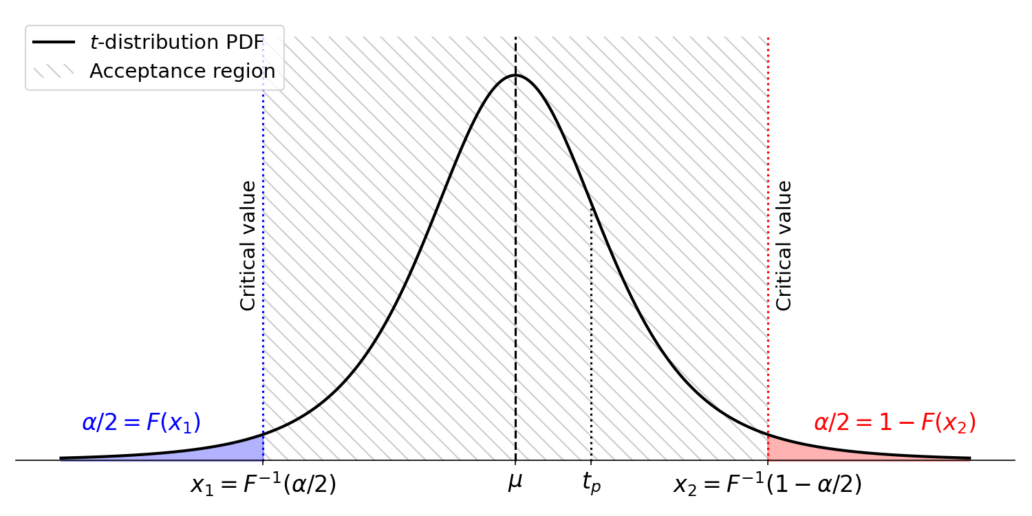
For example, imagine that $b_p = 0$, $t_p = 1$, $\alpha=0.05$, and $N-P=30$. We want to compute the critical values, $x_1$ and $x_2$. We can do this using the CDF $F$ and the inverse CDF $F^{-1}$:

$\begin{aligned} \alpha/2 &= F(x_1) &\implies x_1 &= F^{-1}(0.05/2), \\ \alpha/2 &= 1 - F(x_2) &\implies x_2 &= F^{-1}(1 - 0.05/2). \end{aligned} \tag{11}$

We can then compute $x_1$ and $x_2$ to see if $t_p = 1$ is outside of the acceptance region. Historically, before easy access to statistical software, one would look up the critical values in a $t$-table. However, today, it is easy to quickly compute the critical values, e.g. in Python:

>>> from scipy.stats import t
>>> tdist = t(df=30)
>>> alpha = 0.05
>>> x1 = tdist.ppf(alpha/2)
>>> x2 = tdist.ppf(1 - alpha/2)
>>> (x1, x2)
(-2.042272456301238, 2.0422724563012373)

We can see that $t_p = 1$ is not significant at level $\alpha=0.05$ with $N-P=30$.

$z$-scores vs $t$-statistics

At this point, we have enough of an understanding of $z$-scores and $t$-statistics to say why we typically use $t$-statistics in hypothesis testing for OLS. First, we typically don’t know the population standard deviation $\sigma$. Second, if $N - P$ is sufficiently large, then the $t$-distribution is approximately normal (Figure $2$). Given that both these conditions are often true, it makes sense to just use $t$-statistics by default.

Figure 2. $t$-distribution with varying values for the degrees of freedom parameter (blue lines) versus standard normal distribution (red line).

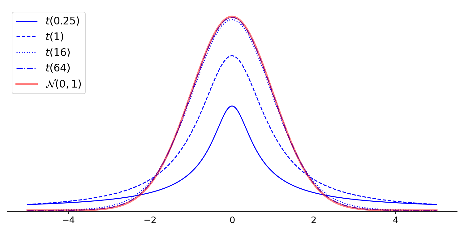
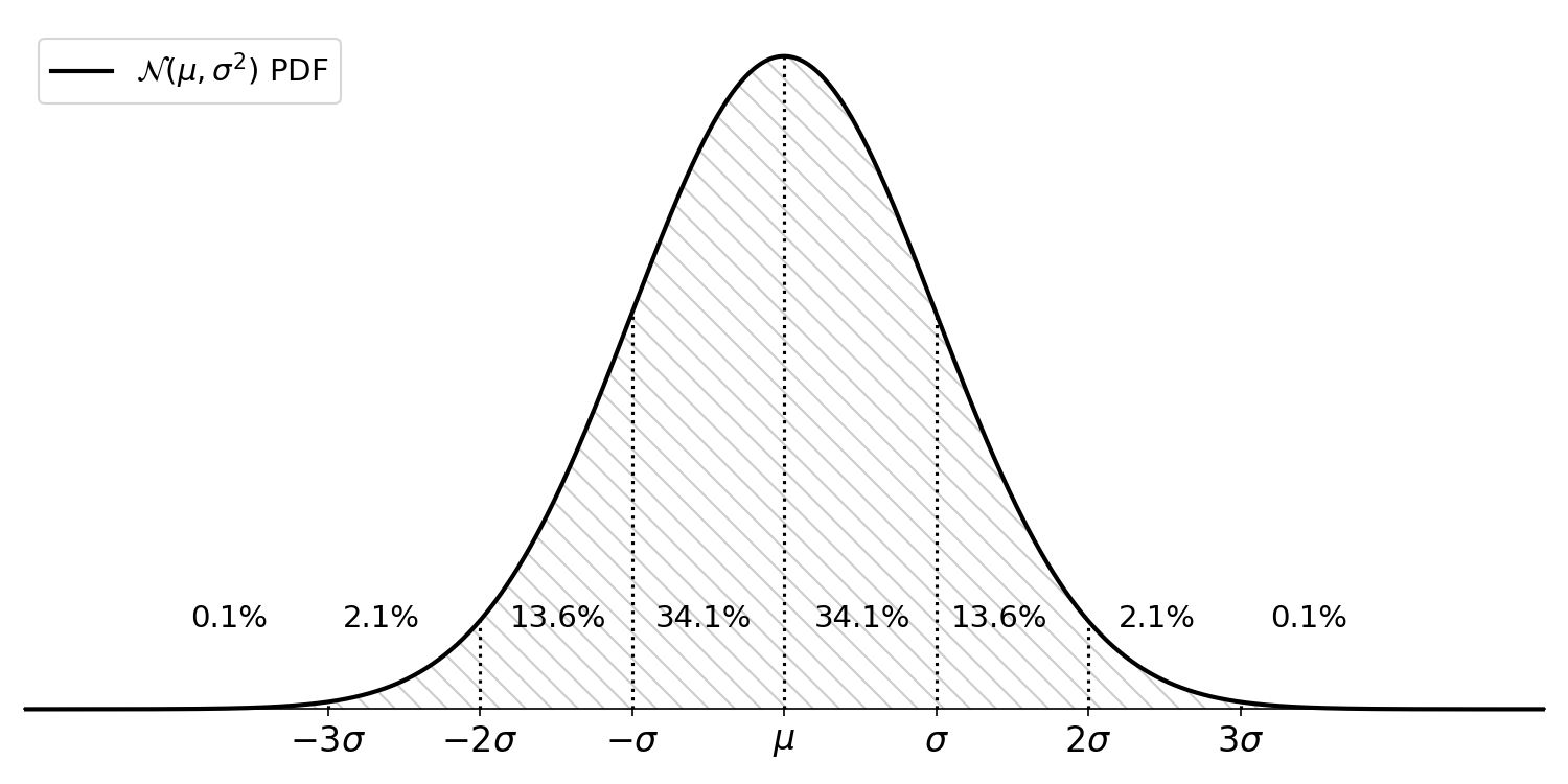
Note that when $N - P$ is reasonably large, where “reasonably large” is traditionally defined as $30$, the $t$-distribution is well-approximated by the standard normal distribution, $\mathcal{N}(0, 1)$. Here, we know that roughly $95\%$ of the mass is within two standard deviations of the mean (Figure $3$). Thus, as a first approximation without using $t$-tables or statistical software, we can say that a $t$-statistic greater than $2\sigma = 2$ is significant when $N - P > 30$.

Figure 3. The normal distribution with mean $\mu$ and standard deviation $\sigma$. Roughly $95\%$ of the mass is within two standard deviations of the mean.

Statistical significance without knowing $\hat{\beta}$

What if we know that the correlation between our regression targets and a single predictor was $\rho_{xy} = 0.1$. Without knowing $\hat{\beta}$, can we compute the minimum number of samples $N$ we need to have a statistically significant inference? In fact, we can. This is a fun result that’s worth knowing about.

In a previous post, I re-derived a standard result that shows that the residual sum of squares (RSS) can be written in terms of the un-normalized sample variance and Pearson’s correlation:

$\textsf{RSS} = S_y^2 (1 - \rho_{xy}^2). \tag{12}$

And the OLS estimator of the variance, $s^2$, can be written in terms of RSS,

$s^2 = \frac{\mathbf{e}^{\top} \mathbf{e}}{N-P} = \frac{\text{RSS}}{N-P} = \frac{S_y^2 (1 - \rho_{xy}^2)}{N-P}. \tag{13}$

Furthermore, we know that $\hat{\beta}$ can be written in terms of the correlation and un-normalized sample standard deviations,

$\hat{\beta} = \rho_{xy} \left( \frac{S_y}{S_x} \right). \tag{14}$

See my previous post on simple linear regression and correlation for a derivation of this fact. Putting this together with Equation $8$ and assuming $b_p = 0$, we can re-write the $t$-statistic as

$\begin{aligned} t &= \frac{\hat{\beta}}{\sqrt{s^2 / S_x^2}} \\ &= \frac{\rho_{xy} \left( S_y / S_x \right)}{\frac{S_y}{S_x} \sqrt{\frac{(1 - \rho_{xy}^2)}{N-P}}} \\ &= \frac{\rho_{xy} \sqrt{N-P}}{\sqrt{1 - \rho_{xy}^2}} \end{aligned} \tag{15}$

In simple linear regression, $P=1$. And we know $\rho_{xy} = 0.1$, so we have

$0.1 \frac{\sqrt{N-1}}{\sqrt{1 - 0.01}} \tag{16}$

So for a confidence level $\alpha = 0.05$, we need $N \approx 400$ samples to have a statistically significant result. This section is a bit tangential to the main ideas of this post, but this is a fun result.

Conclusion

In OLS, assuming normal error terms implies our estimated coefficients are normally distributed. This allows us to construct standard scores and $t$-statistics with well-defined distributions. We can use these test statistics to back out $p$-values, which quantify the probability that we observe a result at least as extreme as $\hat{\beta}_p$ under the null hypothesis.

Acknowledgements

I thank Mattia Mariantoni for pointing out a typo in Equation $15$.

Appendix

A1. Proof that $t$-statistics are $t$-distributed with $N-P$ degrees of freedom

This proof is from (Hayashi, 2000). We can write the $t$-statistic for the $p$-th predictor in Equation $9$ in terms of its $z$-score:

$\begin{aligned} t_p &= \frac{\hat{\beta}_p - b_p}{\sqrt{\sigma^2 [(\mathbf{X}^{\top} \mathbf{X})^{-1}]_{pp}}} \cdot \sqrt{\frac{\sigma^2}{s^2}} \\ &= z_p \cdot \sqrt{\frac{\sigma^2}{s^2}} \\ &\stackrel{\star}{=} \frac{z_p}{\sqrt{\frac{\mathbf{e}^{\top} \mathbf{e} / (N-P)}{\sigma^2}}} \\ &\stackrel{\dagger}{=} \frac{z_p}{\sqrt{\frac{q}{\sigma^2}}}. \end{aligned} \tag{A1.1}$

Step $\star$ uses the definition of $s^2$ (Equation $7$). Step $\dagger$ introduces a new variable, $q \triangleq \mathbf{e}^{\top} \mathbf{e} / \sigma^2$.

Now the logic of the proof is as follows. First, we know that $z_p$ has distribution $\mathcal{N}(0, 1)$. We will then show that $q \mid \mathbf{X} \sim \chi^2(N - P)$, or $q$ conditioned on the predictors is chi-squared distributed with $N - P$ degrees of freedom. Next, we will prove that, conditional on $\mathbf{X}$, $z_p$ and $q$ are independent. This immediately implies that $t_p$ is $t$-distributed, since the $t$-distribution is a ratio distribution arising from a normal random variable divided by an independent chi-distributed (or square root of a chid-squared-distributed) random variable.

Step 1. $q \mid \mathbf{X} \sim \chi^2(N - P)$

The proof that the quadratic form in Equation $\text{A1.4}$ below is chi-squared is from here. A chi-squared distributed random variable with $K$ degrees of freedom is the distribution of the sum of $K$ independent standard normal random variables, each squared. Formally, if $z_1, \dots, z_K$ are i.i.d. from $\mathcal{N}(0, 1)$, then $g$ where

$g \triangleq \sum_{k=1}^K z_k^2, \tag{A1.2}$

is chi-squared distributed. We want to show that

$q = \frac{\mathbf{e}^{\top} \mathbf{e}}{\sigma^2} \tag{A1.3}$

is chi-squared distributed. We saw in a previous post (see Equation $17$ here) that

$\mathbf{e}^{\top} \mathbf{e} = \boldsymbol{\varepsilon}^{\top} \mathbf{M} \boldsymbol{\varepsilon}, \tag{A1.4}$

where $\mathbf{M}$ is the residual maker matrix (see Equation $12$ here for a definition). Since $\mathbf{M} = \mathbf{I} - \mathbf{H}$ and since $\mathbf{H}$ is symmetric (see Equation $A2.2$ here), then clearly $\mathbf{M}$ is symmetric. Thus, $\mathbf{M}$ is diagonalizable with an orthogonal matrix $\mathbf{P}$,

$\mathbf{P}^{\top} \mathbf{M} \mathbf{P} = \boldsymbol{\Lambda} = \begin{bmatrix} \lambda_1 & & & \\ & \lambda_2 & & \\ & & \ddots & \\ & & & \lambda_N \end{bmatrix}. \tag{A1.5}$

Since $\mathbf{M}$ is idempotent, it’s eigenvalues are either zero or one, and the number of non-zero eigenvalues is equal to the rank of $\mathbf{M}$. Now consider the distribution of

$\mathbf{v} \triangleq \mathbf{P}^{\top} \boldsymbol{\varepsilon}. \tag{A1.6}$

Since $\boldsymbol{\varepsilon}$ is normally distributed, and since $\mathbf{P}$ is a linear map, we know that $\mathbf{v}$ is normally distributed. The normal distribution is fully specified by its mean and variance, which for $\mathbf{v}$ are

$\begin{aligned} \mathbb{E}[\mathbf{v}] &= \mathbb{E}[\mathbf{P}^{\top} \boldsymbol{\varepsilon}] \\ &= \mathbf{P}^{\top} \mathbb{E}[\boldsymbol{\varepsilon}] \\ &= \mathbf{0}, \\\\ \mathbb{V}[\mathbf{v}] &= \mathbb{V}[\mathbf{P}^{\top} \boldsymbol{\varepsilon}] \\ &= \mathbf{P}^{\top} \mathbb{V}[ \boldsymbol{\varepsilon}] \mathbf{P} \\ &= \mathbf{P}^{\top} \left( \sigma^2 \mathbf{I} \right) \mathbf{P} \\ &= \sigma^2 \mathbf{I}. \end{aligned} \tag{A1.7}$

So we have shown that

$\mathbf{v} \sim \mathcal{N}(\mathbf{0}, \sigma^2 \mathbf{I}). \tag{A1.8}$

Now we can write $q$ in Equation $\text{A1.3}$ in terms of $\mathbf{v}$,

$\begin{aligned} q &= \frac{\mathbf{e}^{\top} \mathbf{e}}{\sigma^2} \\ &= \frac{\boldsymbol{\varepsilon}^{\top} \mathbf{M} \boldsymbol{\varepsilon}}{\sigma^2} \\ &= \frac{\mathbf{v}^{\top} \mathbf{P}^{\top} \mathbf{M} \mathbf{P} \mathbf{v}}{\sigma^2} \\ &= \frac{1}{\sigma^2} \mathbf{v}^{\top} \boldsymbol{\Lambda} \mathbf{v}. \end{aligned} \tag{A1.9}$

As we said above, since $\mathbf{M}$ is idempotent, it’s eigenvalues are either zero or one, and it has $K \triangleq \text{rank}(\mathbf{M})$ non-zero eigenvalues. So the last line of Equation $\text{A1.9}$ can be written as

$q = \frac{1}{\sigma^2} \mathbf{v}^{\top} \boldsymbol{\Lambda} \mathbf{v} = \frac{1}{\sigma^2} \sum_{k=1}^K v_k^2 = \sum_{k=1}^K \left( \frac{v_k}{\sigma} \right)^2. \tag{A1.10}$

Since each $v_i / \sigma \sim \mathcal{N}(0, 1)$, then $q$ is chi-squared distributed with $K$ degrees of freedom. We saw in a previous post that $K = N - P$ (see Equation $24$ here).

Step 2. $z_p$ and $q$ are independent given $\mathbf{X}$

We want to prove that $z_p$ and $q$ are independent. We’ll do this indirectly, by proving that $\hat{\boldsymbol{\beta}}$ and $\mathbf{e}$ are jointly Gaussian and therefore independent. Since $z_p$ is a function of $\hat{\beta}$ and $q$ is a function of $\mathbf{e}$, this would imply that $z_p$ and $q$ are independent.

The noise terms $\boldsymbol{\varepsilon}$ are multivariate normal,

$\boldsymbol{\varepsilon} \sim \mathcal{N}(\mathbf{0}, \sigma^2 \mathbf{I}). \tag{A1.11}$

Furthermore, both the OLS estimator $\hat{\boldsymbol{\beta}}$ and the residuals $\mathbf{e}$ are linear functions of $\boldsymbol{\varepsilon}$. To see this, recall that we proved the following relationship about the sampling error $\hat{\boldsymbol{\beta}} - \boldsymbol{\beta}$:

$\hat{\boldsymbol{\beta}} - \boldsymbol{\beta} = (\mathbf{X}^{\top} \mathbf{X})^{-1} \mathbf{X}^{\top} \boldsymbol{\varepsilon}. \tag{A1.12}$

(See Equation $8$ here.) Then we can write both $\hat{\boldsymbol{\beta}}$ and $\mathbf{e}$ as

$\begin{aligned} \hat{\boldsymbol{\beta}} &= (\mathbf{X}^{\top} \mathbf{X})^{-1} \mathbf{X}^{\top} \boldsymbol{\varepsilon} + \boldsymbol{\beta}, \\ \\ \mathbf{e} &= \mathbf{y} - \mathbf{X} \hat{\boldsymbol{\beta}} \\ &= \mathbf{X} \boldsymbol{\beta} + \boldsymbol{\varepsilon} - \mathbf{X} (\mathbf{X}^{\top} \mathbf{X})^{-1} \mathbf{X}^{\top} \boldsymbol{\varepsilon} + \boldsymbol{\beta}. \end{aligned} \tag{A1.13}$

So both $\hat{\boldsymbol{\beta}}$ and $\mathbf{e}$ are normal. Now a necessary and sufficient condition for $\hat{\boldsymbol{\beta}}$ and $\mathbf{e}$ to be jointly Gaussian is that for every pair of scalars $(a, b)$, the linear combination $a \hat{\boldsymbol{\beta}} + b \mathbf{e}$ is normal. We have:

$\begin{aligned} a \hat{\boldsymbol{\beta}} + b \mathbf{e} &= a \left[ (\mathbf{X}^{\top} \mathbf{X})^{-1} \mathbf{X}^{\top} \boldsymbol{\varepsilon} + \boldsymbol{\beta} \right] + b \left[ \mathbf{X} \boldsymbol{\beta} + \boldsymbol{\varepsilon} - \mathbf{X} (\mathbf{X}^{\top} \mathbf{X})^{-1} \mathbf{X}^{\top} \boldsymbol{\varepsilon} + \boldsymbol{\beta} \right] \\ &= a (\mathbf{X}^{\top} \mathbf{X})^{-1} \mathbf{X}^{\top} \boldsymbol{\varepsilon} + a \boldsymbol{\beta} + b \mathbf{X} \boldsymbol{\beta} + \boldsymbol{\varepsilon} - b \mathbf{X} (\mathbf{X}^{\top} \mathbf{X})^{-1} \mathbf{X}^{\top} \boldsymbol{\varepsilon} + b \boldsymbol{\beta} \end{aligned} \tag{A1.14}$

This is clearly Gaussian, since $\boldsymbol{\varepsilon}$ is the only random quantity, and the rest of the terms are linear functions or scalars. Thus, conditional on $\mathbf{X}$, $\hat{\boldsymbol{\beta}}$ and $\mathbf{e}$ and are jointly normal and therefore independent. Thus, $z_p$ and $q$ are independent.

Taken together, steps $1$ and $2$ prove that the $t$-statistic is $t$-distributed with $N-P$ degrees of freedom.