Understanding Moments

While drafting another post, I realized that I didn’t fully understand the idea of a distribution’s moments. I could write down the equation for the $k$th moment of a random variable $X$ with a density function $f(x)$,

$\mu_k = \mathbb{E}[X^k] = \int_{-\infty}^{\infty} x^k f(x) \text{d}x, \tag{1}$

and I understood that the first moment is a random variable’s mean, the second (central moment) is its variance, and so forth. Yet the concept felt slippery because I had too many unanswered questions. Why is it called a “moment”? Is it related to the concept of a moment in physics? Why do the first four moments—mean, variance, skewness, and kurtosis—have commonly used names but higher-order moments do not? Is there a probabilistic interpretation of the seventy-second moment? Why does a moment-generating function uniquely specify a probability distribution? The goal of this post is to explore these questions in detail.

This post is long, and I spent many hours writing it. However, I have consistently found that the most time-consuming blog posts are typically those that I needed to write the most. My guess is that this is because foundational ideas often touch many different topics, and understanding them is an iterative process. By this metric, moments are truly foundational.

As an outline, I begin by discussing the etymology of the word “moment” and discussing some terminology such as types of moments. I then walk through the first five moments—total mass, mean, variance, skewness, and kurtosis—in detail. I then attempt to generalize what we’ve learned in those sections to higher moments. I conclude with moment-generating functions.

Movement and shape

My first question about moments was basic: why are they called “moments”? I am clearly not the first person to have thought about this. According to Wiktionary, the words “moment” and “momentum” are doublets or etymological twins, meaning that they are two words in a language with the same etymological root. Both come from the Latin word “movimentum,” meaning to move, set in motion, or change. Today, a “moment” often refers to an instant in time, but we can guess at the connection to movement. For example, we might say things like, “It was a momentous occasion,” or, “The game was her big moment.” In both cases, the notion of time and change are intertwined.

This probably explains the origin of “moment” in physics. In physics, the moment of inertia is a measure of rotational inertia or how difficult it is to change the rotational velocity of an object. A classic example of the moment of inertia is moving a pencil: spinning a pencil about its short axis, say by pushing on the lead point, requires a different amount of force than rolling it about the long axis. This is because the force required is related to how the mass of the pencil is distributed about the axis of rotation.

That last sentence about how mass is distributed about an axis starts to hint at how early probabilists might have landed on the word “moment” to describe distributions—or rather, why they thought “moment of inertia” was a good analogy. There appears to be a thread from the Latin word for setting in motion to the physicist’s notion of changing an object’s rotational velocity to finally the probabilist’s notion of how probability mass is distributed.

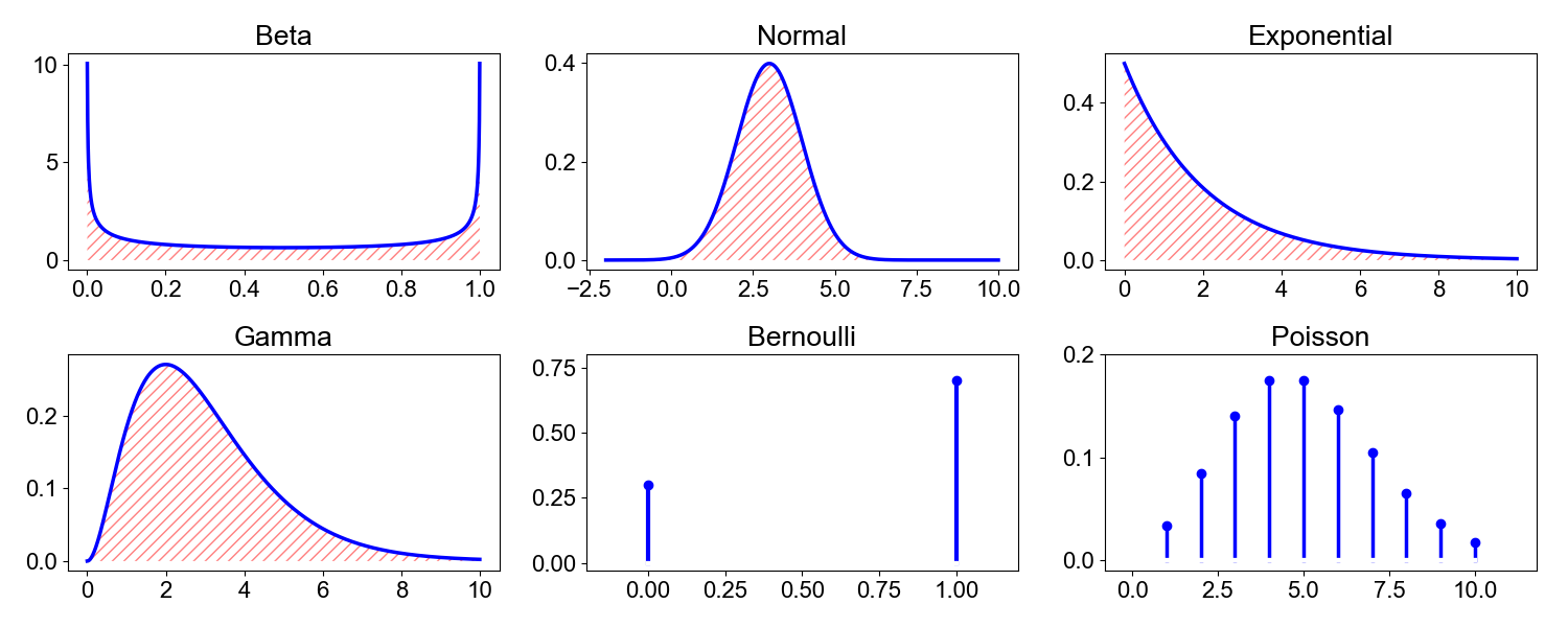
This actually makes a lot of sense because, as we will see, moments quantify three parameters of distributions: location, shape, and scale. By convention, we plot distributions with their support (values that do not have probability zero) on the $x$-axis and each supported value’s probability on the $y$-axis. A distribution’s location refers to where its center of mass is along the $x$-axis. By convention, a mean-centered distribution has a center of mass at zero. The scale refers to how spread out a distribution is. Scale stretches or compresses a distribution along the $x$-axis. Finally, the shape of a distribution refers to its overall geometry: is the distribution bimodal, asymmetric, heavy-tailed? As a preview of the next sections, the first moment describes a distribution’s location, the second moment describes its scale, and all higher moments describe its shape.

Many distributions have parameters that are called “location”, “scale”, or “shape” because they control their respective attributes, but some do not. For example, the Poisson’s parameter is typically called “rate”, and increasing the rate increases the location and scale and changes the shape. In such cases, the terms “location”, “scale”, and “shape” still make sense as adjectives.

Types of moments

With the hunch that “moment” refers to how probability mass is distributed, let’s explore the most common moments in more detail and then generalize to higher moments. However, first we need to modify $(1)$ a bit. The $k$th moment of a function $f(x)$ about a non-random value $c$ is

$\mathbb{E}[(X - c)^k] = \int_{-\infty}^{\infty} (x - c)^k f(x) \text{d}x. \tag{2}$

This generalization allows us to make an important distinction: a raw moment is a moment about the origin ($c = 0$), and a central moment is a moment about the distribution’s mean ($c = \mathbb{E}[X]$). If a random variable $X$ has mean $\mu_x$, then its $k$th central moment is

$m_k = \mathbb{E}[(X - \mu_x)^k] = \int_{-\infty}^{\infty} (x - \mu_x)^k f(x) \text{d}x. \tag{3}$

Central moments are useful because they allow us to quantify properties of distributions in ways that are location-invariant. For example, we may be interested in comparing the variability in height of adults versus children. Obviously, adults are taller than children on average, but we want to measure which group has greater variability while disregarding the absolute heights of people in each group. Central moments allow us to perform such calculations.

Finally, the $k$th standardized moment is typically defined as the $k$th central moment normalized by the standard deviation raised to the $k$th power,

$\bar{m}_k = \frac{m_k}{\sigma_k} = \mathbb{E}\left[\left(\frac{X - \mu_x}{\sigma_x}\right)^k\right], \tag{4}$

where $m_k$ is defined as in $(3)$, and $\sigma_k$ is the $k$th power of the standard deviation of $X$,

$\sigma_k = \sigma_x^k = \left( \sqrt{\mathbb{E}[(X - \mu_x)^2]} \right)^k. \tag{5}$

Note that $(4)$ is only well-defined for distributions whose first two moments exist and whose second moment is non-zero. This holds for most distributions of interest, and we will assume it is true for the remainder of the post. Standardization makes the moment both location- and scale-invariant. Why might we care about scale invariance? As we will see, the third, fourth, and higher standardized moments quantify the relative and absolute tailedness of distributions. In such cases, we do not care about how spread out a distribution is, but rather how the mass is distributed along the tails.

Finally, a sample moment is an unbiased estimator of its respective raw, central, or standardized moment. For example, the sample moment of $(2)$ is

$\tilde{m}_k = \frac{1}{N} \sum_{n=1}^{N} (x_n - c)^k. \tag{6}$

I use uppercase $X$ to denote a random variable and lowercase $x_n$ to denote the $n$th realization from $N$ samples. Recall that, given a statistical model, parameters summerize data for an entire population, while statistics summarize data from a sample of the population. We compute the former exactly using a statistical model and estimate it from data using the latter. For example, if we assume that $X \sim \mathcal{N}(\mu_x, \sigma_x^2)$, then the first raw moment is $\mathbb{E}[X] = \mu_x$, and we estimate it with the sample mean.

There’s a lot to unpack here. To summarize nomenclature and my notation, we have:

$\begin{aligned} \mu_k &= \mathbb{E}[X^k] && \text{$k$th raw moment} \\ m_k &= \mathbb{E}[(X - \mu_k)^k] && \text{$k$th central moment} \\ \\ \bar{m}_k &= \mathbb{E}\left[\left(\frac{X - \mu_x}{\sigma_x}\right)^k\right] && \text{$k$th standardized moment} \\ \tilde{m}_k &= \frac{1}{N} \sum_{n=1}^{N} (X_n - c)^k. && \text{$k$th sample moment about $c$} \end{aligned} \tag{7}$

Now let’s discuss the first five moments in order: total mass, mean, variance, skewness, and kurtosis. Then I’ll attempt a synthesis before ending on moment-generating functions.

Total mass

Since $x^0 = 1$ for any number $x$, the zeroth raw, central, and standardized moments are all

$\mu_0 = m_0 = \bar{m}_0 = \int_{-\infty}^{\infty} (\dots)^0 f(x) \text{d}x = \int_{-\infty}^{\infty} f(x) \text{d}x = 1, \tag{8}$

where $(\dots)$ denotes $x$, $(x - \mu_x)$, or $(x - \mu_x) / \sigma_x$. In other words, the zeroth moment captures the fact that probability distributions are normalized quantities, that they always sum to one regardless of their location, scale, or shape (Figure $1$).

Figure 1. Beta, normal, exponential, gamma, Bernoulli, and Poisson distributions, each with a total mass of one.

Another way to think about $(8)$ is that the probability that at least one of the events in a sample space will occur is $1$. Thus, the zeroth moment captures Kolmogorov’s second probability axiom.

Mean

The first raw moment, the expectation of $X$, is

$\mu_1 = \mu_x = \mathbb{E}[X] = \int_{-\infty}^{\infty} x f(x) \text{d}x. \tag{9}$

We can think about the first moment in a few ways. Typically, the expectation of $X$ is introduced to students as the long-run average of $X$. For example, if $X$ is the outcome of a roll of a fair six-sided die, then its expectation is

$\mathbb{E}[X] = 1 \cdot \frac{1}{6} + 2 \cdot \frac{1}{6} + 3 \cdot \frac{1}{6} + 4 \cdot \frac{1}{6} + 5 \cdot \frac{1}{6} + 6 \cdot \frac{1}{6} = 3.5. \tag{10}$

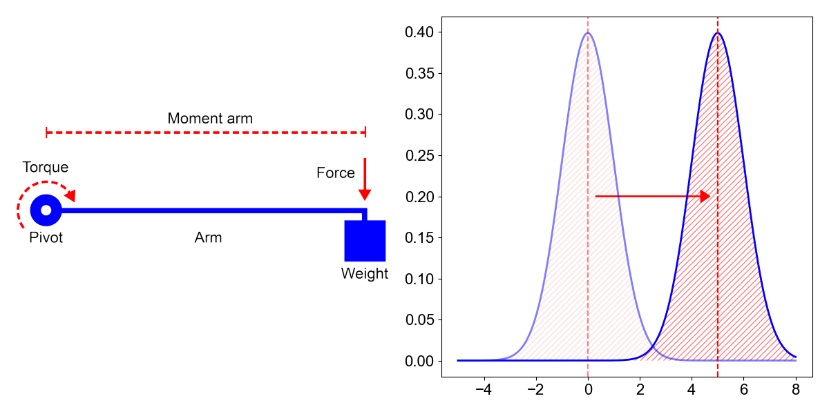
If we repeatedly roll a die many times, the finite average of the die rolls will slowly converge to the expected value (Figure $2$, left), hence the name “expectation”. Another way to think about the first moment is that it is that it is the center of mass of a probability distribution. In physics, the center of mass is the point at which all the torques due to gravity sum to zero. Since torque is a function of both the force (gravity) and moment arm (distance from the fulcrum), it makes sense that the mean-as-center-of-mass interpretation suggests the probabiltiy mass is perfectly balanced on the mean (Figure $2$, right).

Figure 2. (Left) Expectation as an average: the convergence of the average outcome from rolling a fair six-sided die. (Right) Expectation as a center of mass: the mass of the probability distribution is balanced upon the expected value; plotted is a beta distribution with parameters $\alpha = 2$ and $\beta = 5$. The fulcrum is placed at the mean, $\alpha / (\alpha + \beta) = 2 / 7$.

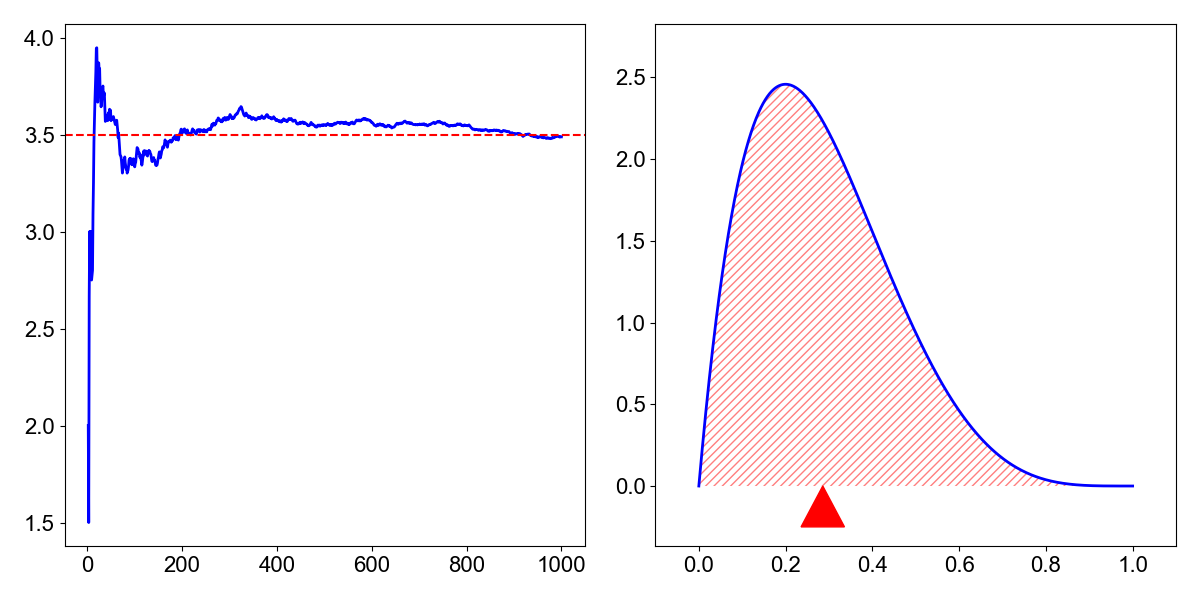
However, there’s a third way to think about the first moment, and it’s the one that I think is most useful for understanding moments generally: the first moment tells us how far away from the origin the center of mass is. I like this interpretation because it is analogous to a moment arm in mechanics, which is the length of an arm between an axis of rotation and a force acting perpendicularly against that arm (Figure $3$, left). For example, if you open a door by its handle, the moment arm is the roughly the width of the door. The first moment of a distribution is a bit like a moment arm. It measures the distance between the distribution’s center of mass and the origin (Figure $3$, right).

Figure 3. (Left) A moment arm is the length between a pivot point and a force. (Right) The first moment is the distance between the origin point and the center of mass.

This is an important interpretation because it will help justify central moments in the next sections. Subtracting each value of the support of $X$ by $\mathbb{E}[X]$ can be visualized as simply shifting the distribution such that its mean is now zero. This gives us a way to normalize distributions with different means so that we can compare their scales and shapes while disregarding the absolute values the random variables can take. Again, think about how you would compare variability in heights of children versus adults while ignoring the fact that adults are obviously taller.

Typically, the first moment of a distribution is always the first raw moment. The first central and standardized moments are less interesting because they are always zeros:

$\mathbb{E}[X - \mu_x] = \mathbb{E}[X] - \mathbb{E}[\mu_x] = \mu_x - \mu_x = 0. \tag{11}$

Variance

The second moment is where, in my mind, things start to get a bit more interesting. Typically, people are interested in the second central moment, rather than the second raw moment. This is called the variance of a random variable $X$, denoted $\mathbb{V}[X]$,

$m_2 = \mathbb{V}[X] = \int_{-\infty}^{\infty} (x - \mu_x)^2 f(x) \text{d}x. \tag{12}$

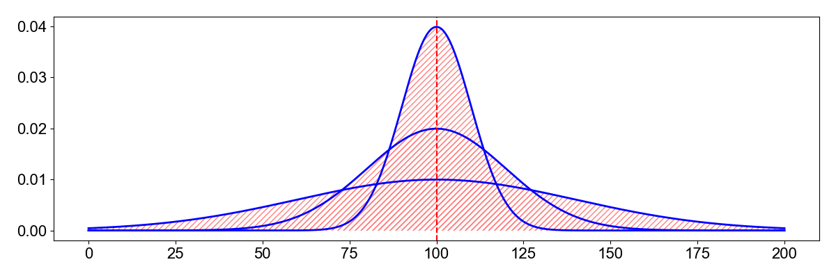
The second central moment increases quadratically as mass gets further away from the distribution’s mean. In other words, variance captures how spread out a distribution is or its scale parameter. Points that are further away from the mean than others are penalized disproportionally. High variance means a wide distribution (Figure $4$), which can loosely be thought of as a “more random” random variable; and a random sample from a distribution with a second central moment of zero always takes the same value, i.e. it is non-random. Again, the loose connection to “moment of inertia” seems clear in that the second central moment captures how wide a distribution is.

Figure 4. Three normal distributions with the same first moment but different variances. Bigger variance means a wider distribution, meaning higher variability in outcomes.

Why are we interested in the second central moment, rather than the second raw moment? Imagine we wanted to compare two random variables, $X$ and $Y$. If the values that $X$ can take are larger than the values that $Y$ can take, the second raw moment could be bigger, regardless of how far away the realizations are from the mean of the distribution. This idea maps onto my example of comparing the variability in height of adults versus children. If we first subtract the mean before calculating the second moment, we can compare each distribution’s relative spread while ignoring its location.

This distinction is easy to demonstrate in code:

import numpy.random as npr

# `X` has larger values on average, but `Y` has higher variability in values.
X = npr.normal(10, 1, size=1000)
Y = npr.normal(0, 2, size=1000)

# So `X` has a larger second raw moment.
mx = (X**2).mean()
my = (Y**2).mean()
print(f'{mx:.2f}\t{my:.2f}')  # 102.32  3.96

# But `Y` has a larger second central moment (variance).
mx = X.var()
my = Y.var()
print(f'{mx:.2f}\t{my:.2f}')  # 1.06    3.96

We are less interested in the second standardized moment because it is always one,

$\bar{m}_2 = \frac{\mathbb{E}[(X - \mu)^2]}{(\sqrt{\mathbb{E}[(X - \mu)^2]})^2} = 1. \tag{13}$

That said, there is an interesting connection between the variance or second central moment and the second raw moment:

$\begin{aligned} \mathbb{V}[X] &= \mathbb{E}[(X - \mathbb{E}[X])^2] \\ &= \mathbb{E}[X^2 + \mathbb{E}[X]^2 - 2 X \mathbb{E}[X]] \\ &= \mathbb{E}[X^2] + \mathbb{E}[X]^2 - 2 \mathbb{E}[X] \mathbb{E}[X] \\ &= \mathbb{E}[X^2] - \mathbb{E}[X]^2. \end{aligned} \tag{14}$

Since $\mathbb{E}[X]$ is non-random, $\mathbb{E}[X]^2$ is non-random. This implies that the second central moment is equivalent to the second raw moment up to a constant. In fact, since $\mathbb{E}[X]^2$ is nonnegative, we can see that the second moment attains the smallest possible value when taken around the first moment.

Skewness

The third standardized moment, called skewness, measures the relative size of the two tails of a distribution,

$\bar{m}_3 = \mathbb{S}[X] = \mathbb{E}[Z^3] = \mathbb{E}\left[\left(\frac{X - \mu_x}{\sigma_x}\right)^3\right], \tag{15}$

where $Z$ is the standard score or $z$-score:

$Z = \frac{X - \mu_x}{\sigma_x}. \tag{16}$

To see how $(15)$ quantifies the relative size of the two tails, consider this: any data point less than a standard deviation from the mean (i.e. data near the center) results in a standard score less than $1$; this is then raised to the third power, making the absolute value of the cubed standard score even smaller. In other words, data points less than a standard deviation from the mean contribute very little to the final calculation of skewness. Since the cubic function preserves sign, if both tails are balanced, the skewness is zero. Otherwise, the skewness is positive for longer right tails and negative for longer left tails.

You might be tempted to think that $(15)$ quantifies symmetry, but this is a mistake. While a symmetric distribution always has a skewness of zero, the opposite claim is not always true: a distribution with zero skewness may be asymmetric. We’ll see an example at the end of this section.

Figure 5. (Left) Negative or left skewness. (Right) Positive or right skewness.

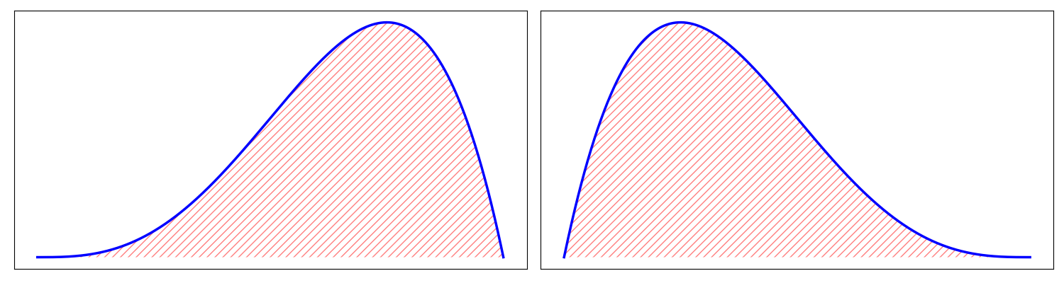
The above reasoning makes the terminology around skewness fairly intuitive. A left skewed or negatively skewed distribution has a longer left tail and $(15)$ is negative (Figure $5$, left). A right skewed or positively skewed distribution has a longer right tail and $(15)$ is positive (Figure $5$, right).

To concretize this idea, let’s look at two examples of how the tails dominate the skewness calculation in $(15)$. First, let’s take one thousand samples from the skew normal distribution and compute the percentage of absolute valued standard scores that are within one standard deviation of the mean. As we can see below, roughly $90\%$ of the skewness calculation comes from the tails, despite the tails being less than half of the total mass (Figure $6$, left).

from numpy.random import RandomState
from scipy.stats import skewnorm

rng     = RandomState(seed=0)
X       = skewnorm(a=5).rvs(size=1000, random_state=rng)
Z_abs   = abs((X - X.mean()) / X.std())
s_total = (Z_abs**3).sum()
s_peak  = (Z_abs[Z_abs <  1]**3).sum()
s_tails = (Z_abs[Z_abs >= 1]**3).sum()

print(f'Tails: {s_tails / s_total:.4f}')  # 0.9046
print(f'Peak : {s_peak  / s_total:.4f}')  # 0.0954

Figure 6. (Left) Histogram of one thousand samples of a skew normal distribution with parameter $\alpha = 5$. Light blue bins represent data within one standard deviation of the sample mean. (Right) Probability mass function of a Bernoulli distribution with parameter $p = 0.3$.

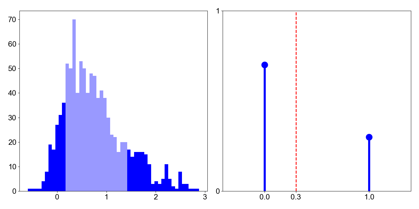
For a second example, consider a Bernoulli random variable, $X \sim \text{Bernoulli}(p)$ where $p < 1/2$. Since $p < 1/2$, clearly $1 - p > p$ (Figure $6$, right). This means that more mass is to the left of the mean, $\mathbb{E}[X] = p$, but it is easy to show that this distribution is right skewed. Using the fact that $\mu_x = p$ and $\sigma_x = \sqrt{p(1-p)}$, let’s compute the third standardized moment:

$\begin{aligned} \mathbb{E}\left[\left(\frac{X - p}{\sqrt{p(1-p)}}\right)^3\right] &= \frac{(1 - p)^3 p + (0 - p)^3 (1 - p)}{[p(1-p)]^{3/2}} \\ &= \frac{(1 - p)^3 p - p^3 (1 - p)}{[p(1-p)]^{3/2}} \\ &= \frac{p (1 - p) (1 - 2p)}{[p(1-p)]^{3/2}} \\ &= \frac{1 - 2p}{[p (1 - p)]^{1/2}} \end{aligned} \tag{17}$

This moment is positive—the distribution is right skewed—if and only if $p < 1/2$, which is true by assumption. Thus, we have a right skewed distribution with more mass to the left of the mean. Again, we see that the smaller mass on the tails dominates the calcuation of skewness.

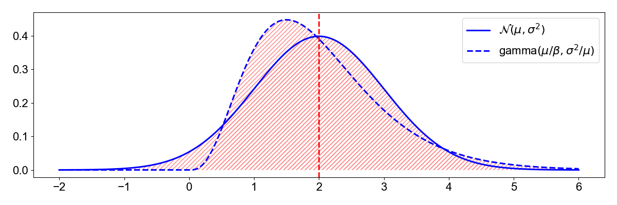
Standardizing the moment in $(15)$ is important because skewness is both location- and scale-invarant. In other words, two distributions can have the same mean and variance but different skewnesses. For example, consider the two random variables in $(18)$,

$\begin{aligned} X &\sim \mathcal{N}(\mu, \sigma^2) \\ Y &\sim \text{gamma}\left(\alpha = \frac{\mu}{\beta}, \beta = \frac{\sigma^2}{\mu}\right). \end{aligned} \tag{18}$

Note that the gamma distribution’s second parameter $\beta$ depends on $\mu$ and $\sigma^2$, and its first parameter $\alpha$ depends on $\mu$ and $\beta$. (Credit to John Cook for this idea.) Using the definitions of mean and variance for these random variables, it is easy to see that

$\begin{aligned} \mathbb{E}[X] &= \mu, & \mathbb{E}[Y] &= \alpha \beta = \frac{\mu}{\beta} \beta = \mu \\ \mathbb{V}[X] &= \sigma^2, & \mathbb{V}[Y] &= \alpha \beta^2 = \mu \beta = \mu \frac{\sigma^2}{\mu} = \sigma^2. \end{aligned} \tag{19}$

However, the normal distribution is always symmetric and has a skewness of zero, while this gamma distribution has a skewness of $2 / \sqrt{\alpha} = 2\sigma / \mu$ (Figure $7$). Thus, we want a metric for skewness that ignores location and scale. This is one reason for taking skewness to be a standardized moment. As a fun aside, note that the gamma distribution will have a skewness approaching zero as $\mu$ increases.

Figure 7. Two distributions with the same mean and variance but different skewnesses: a normal distribution with mean $\mu$ and variance $\sigma^2$ and a gamma distribution with parameters $\alpha = \mu/\beta$ and $\beta = \sigma^2/\mu$.

To see why standardization works for $(15)$, consider the skewness of two random variables, $X$ with mean $\mu_x$ and variance $\sigma_x^2$ and $Y = cX$ for some constant $c > 0$. Then

$\begin{aligned} \mathbb{S}[X] &= \mathbb{E}\left[\left(\frac{X - \mu_x}{\sigma_x}\right)^3\right] \\ &= \frac{c^3}{c^3} \mathbb{E}\left[\left(\frac{X - \mu_x}{\sigma_x}\right)^3\right] \\ &= \mathbb{E}\left[\left(\frac{cX - c\mu_x}{c \sigma_x}\right)^3\right] \\ &= \mathbb{S}[Y]. \end{aligned} \tag{20}$

In words, skewness is invariant to sign-preserving scaling transformations. Note that if $c < 0$, the skewness’s value would be preserved, but the sign would be flipped. And if of course, the mean-centering makes the metric invariant under translation, i.e. if $X = Y+c$ then

$\mathbb{S}[X] = \mathbb{E}\left[\left(\frac{X - \mu_x}{\sigma_x}\right)^3\right] = \mathbb{E}\left[\left(\frac{Y+c - (\mu_y+c)}{\sigma_x}\right)^3\right] = \mathbb{S}[Y]. \tag{21}$

Without this standardization, either the location or scale of the distribution could undesirably affect the calculation of skewness. For example, consider this Python code, which estimates the third raw moment of two exponential random variables that have the same skewness but different locations and the third central moment of two skew normal random variables with the same skewness but different scales:

from numpy.random import RandomState
from scipy.stats import expon, skewnorm

def raw_moment(X, k, c=0):
    return ((X - c)**k).mean()

def central_moment(X, k):
    return raw_moment(X=X, k=k, c=X.mean())

rng = RandomState(seed=0)
sample_size = int(1e6)

# `X` and `Y` have the same skewness but different locations.
# The un-centered moment does not capture this.
dist1 = expon(0, 1)
X = dist1.rvs(size=sample_size, random_state=rng)
dist2 = expon(2, 1)
Y = dist2.rvs(size=sample_size, random_state=rng)
print(f'skew1: {dist1.stats(moments="s")}')  # 2.0
print(f'skew2: {dist2.stats(moments="s")}')  # 2.0
print(f'raw1 : {raw_moment(X, k=3):.2f}')    # 6.03
print(f'raw2 : {raw_moment(Y, k=3):.2f}')    # 38.04

# `X` and `Y` have the same skewness but different scales.
# The central but not standardized moment does not capture this.
dist1 = skewnorm(a=2, loc=0, scale=1)
X = dist1.rvs(size=sample_size, random_state=rng)
dist2 = skewnorm(a=2, loc=0, scale=4)
Y = dist2.rvs(size=sample_size, random_state=rng)
print(f'skew1   : {dist1.stats(moments="s")}')    # 0.45382556395938217
print(f'skew2   : {dist2.stats(moments="s")}')    # 0.45382556395938217
print(f'central1: {central_moment(X, k=3):.2f}')  # 0.16
print(f'central2: {central_moment(Y, k=3):.2f}')  # 10.11

Clearly, in both cases the raw and central moments do not correctly quantify the relative skewness of the distributions, hence the standardization in $(15)$.

Finally, let’s look explore why “symmmetry” is a bad analogy for skewness by looking at an example of an asymmetric distribution with a skewness of zero. This example is borrows from this article by Donald Wheeler. Following the notation and results in (Dey et al., 2017), a Dagum distributed random variable $X$ has a probability density function

$f(x; \beta, \lambda, \delta) = \beta \lambda \delta x^{-(\delta + 1)} \left( 1 + \lambda x^{-\delta} \right)^{-(\beta + 1)}, \quad \beta > 0, \lambda > 0, \delta > 0, x > 0. \tag{22}$

Using the results in section $2.4$ of Dey, we see that the $k$th moment is:

$\mathbb{E}[X^k] = \lambda^{k / \delta} \frac{\Gamma(1 - k/\delta)\Gamma(\beta + k/\delta)}{\Gamma(\beta)}. \tag{23}$

And for $k = 3$, we can compute the skewness of the Dagum distribution (or any distribution) using just the raw moments,

$\bar{m}_3 = \frac{\mathbb{E}[X^3] - 3 \mathbb{E}[X] (\mathbb{E}[X^2] - \mathbb{E}[X]^2) - \mathbb{E}[X]^3}{(\mathbb{E}[X^2] - \mathbb{E}[X]^2)^{3/2}}. \tag{24}$

See A1 for a derivation of this skewness decomposition. If we set $\lambda = 1$, and use SciPy’s excellent minimize function, we can find optimal parameters that minimize the absolute value of the skewness (Figure $8$):

$\begin{aligned} \beta = 0.23624499839 &\quad \delta = 10.45787742085 \\ &\Downarrow \\ \mathbb{S}[X] &= 0.00000000047 \end{aligned} \tag{25}$

See A2 for Python code to reproduce the optimization.

Figure 8. An asymmetric Dagum distribution with zero skewness; parameters are $\beta = 0.23624499839$ and $\delta = 10.45787742085$.

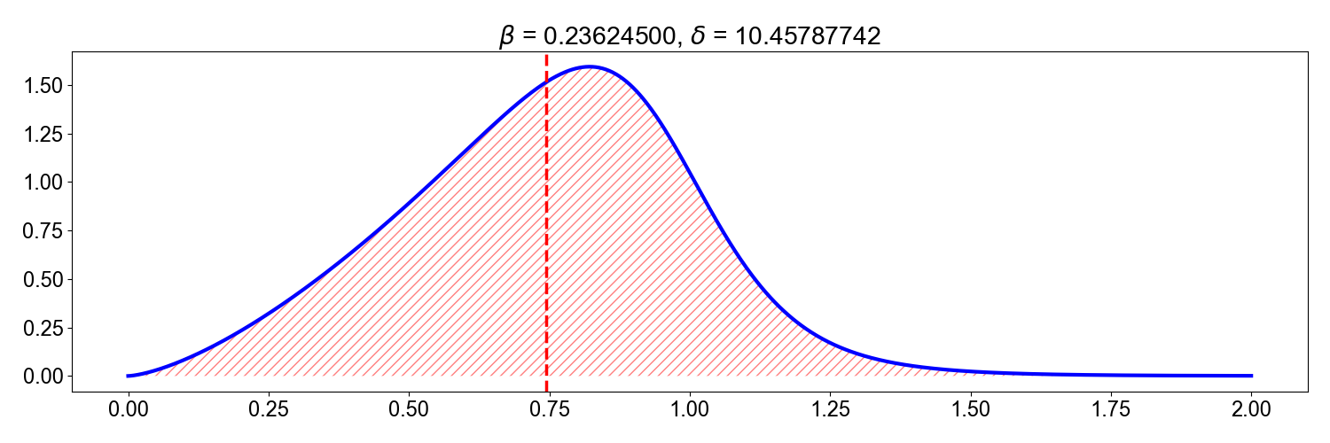
This example is contrived, but it is not hard to imagine real data taking the shape of Figure $8$. Thus, I think it is better to always say that skewness captures “relative tailedness” rather than “asymmetry”.

Kurtosis

While skewness is a measure of the relative size of the two tails and is positive or negative depending on which tail is larger, kurtosis is a measure of the combined size of the tails relative to whole distribution. There are a few different ways of measuring this, but the typical metric is the fourth standardized moment,

$\bar{m}_4 = \mathbb{K}[X] = \frac{\mu_4}{\sigma_4} = \mathbb{E}\left[\left(\frac{X - \mu}{\sigma}\right)^4\right]. \tag{26}$

Unlike skewness’s cubic term which preserves sign, kurtosis’s even power means that the metric is always positive and that long tails on either side dominate the calculation. Just as we saw with skewness, kurtosis’s fourth power means that standard scores less than $1$—again, data near the peak of the distribution—only marginally contribute to the total calculation. In other words, kurtosis measures tailedness, not peakedness. Again, we standardize the moment because two distributions can have the same mean and variance but different kurtosises (see Figure $10$ below for an example).

Since I approached learning about kurtosis with a blank slate, I did not think of kurtosis as peakedness rather than tailedness. However, a number of resources cautioned against such a mistake, claiming it was a common misinterpretation. See (Darlington, 1970) and (Westfall, 2014) for detailed discussions. In particular, Westfall has a convincing example for how kurtosis is not peakedness, which I’ll replicate here. Consider one thousand random samples from the Cauchy distribution with location $0$ and scale $1$ (Figure $9$).

Figure 9. Histogram of one thousand samples of a Cauchy distribution with location $0$ and scale $1$. Red dots highlight histogram bins that are more than a standard deviation from the mean.

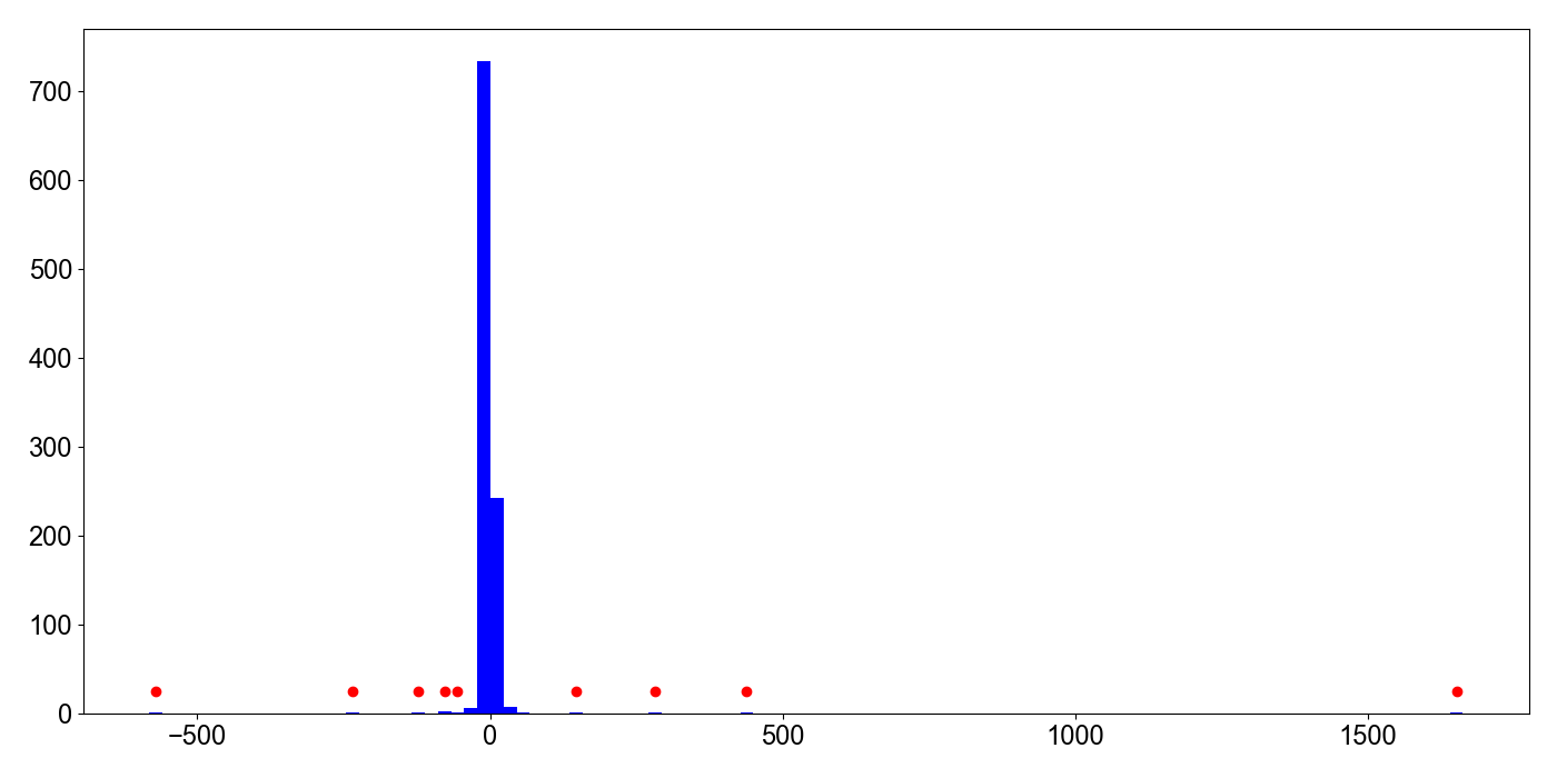
Clearly, the empirical distribution is peaked or pointy, but it also has outliers. We can compute the sample fourth standardized moment $(26)$ and see what percentage of that calculation comes from the peaks versus the tails by separating the calculation of kurtosis by data within or outside of one standard deviation of the mean:

from numpy.random import RandomState
from scipy.stats import cauchy

rng     = RandomState(seed=0)
N       = 1000
X       = cauchy(0, 1).rvs(size=N, random_state=rng)
Z       = (X - X.mean()) / X.std()
k_total = (Z**4).mean()
k_peak  = (Z[abs(Z) <  1]**4).sum() / N
k_tails = (Z[abs(Z) >= 1]**4).sum() / N

print(f'Tails: {k_tails / k_total:.8f}')  # 0.99999669
print(f'Peak : {k_peak  / k_total:.8f}')  # 0.00000331

The result shows that the kurtosis calculation is absolutely dominated by the outliers. Roughly $99\%$ of the total kurtosis comes from the tails.

With the intuition that kurtosis measures tailedness, let’s consider two alternative ways of interpreting it. First, note that the kurtosis any univariate normal is $3$:

$\mathbb{E}\left[ \left(\frac{X-\mu}{\sigma}\right)^4 \right] = \frac{1}{\sqrt{2 \pi}} \int_{-\infty}^{\infty} a^4 \exp\Big\{-\frac{1}{2} a^2\Big\} \text{d}a = 3, \tag{27}$

where $a = (x-\mu)/\sigma$ and $\text{d}a = \text{d}x / \sigma$. See A3 for a complete derivation. So one common re-framing of kurtosis is excess kurtosis,

$\mathbb{K}[X] - 3, \tag{28}$

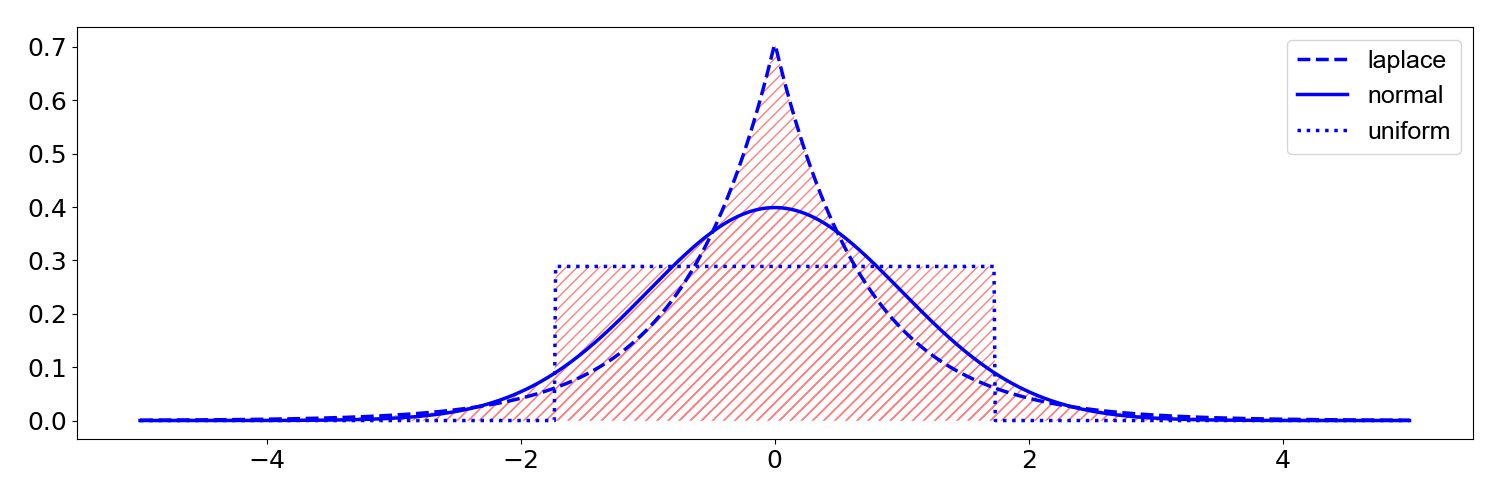
which can be thought of as the tailedness of $X$ relative to the normal distribution. For example, a Laplace distribution with scale parameter $1 / \sqrt{2}$—chosen so that the variance is $1$—has an excess kurtosis of $3$. This means it is “more tailed” than a normal distribution (Figure $9$). Conversely, a uniform distribution with minimum and maximum values of $\pm \sqrt{3}$—again chosen so that the variance is $1$—has an excess kurtosis of $-1.2$. This means it is “less tailed” than a normal distribution (Figure $10$).

Figure 10. Laplace, normal, and uniform distributions with mean $0$ and variance $1$. Respectively, their excess kurtosises are $3$, $0$, and $-1.2$.

As a second interpretation, (Darlington, 1970) and (Moors, 1986) argue that kurtosis can be viewed as the variance of $Z^2$ around its mean of $1$. To see this, consider the fact that

$\begin{aligned} \mathbb{K}[X] &= \mathbb{E}[Z^4] \\ &= \mathbb{V}[Z^2] + \mathbb{E}[Z^2]^2 \\ &\stackrel{\star}{=} \mathbb{V}[Z^2] + \mathbb{V}[Z]^2 \\ &= \mathbb{V}[Z^2] + 1. \end{aligned} \tag{29}$

Step $\star$ holds because

$\mathbb{V}[Z] = \mathbb{E}[Z^2] - \mathbb{E}[Z]^2 \tag{30}$

and $\mathbb{V}[Z] = 1$ and $\mathbb{E}[Z] = 0$ by definition. See A4 for a derivation. In the context of $(29)$, kurtosis can be interpreted as the variance or dispersion of $Z^2$. If the random variable $Z^2$ has low variance, then $X$ has low kurtosis. If $Z^2$ has high variance, then $X$ has high kurtosis.

Generalizing and higher moments

Let’s fix the discussion around standardized moments and synthesize what we have learned so far; then we will generalize to higher moments. I want to finally answer the question: “Is there a probabilistic interpretation of the seventy-second moment?”

To review, the zeroth standardized moment is always $1$ because raising anything to the zeroth power is $1$ and probability distributions are normalized. The first standardized moment is always $0$ because we subtract the mean, while the second standardized moment is always $1$ because we then divide by the variance. The third standardized moment, skewness, measures the relative size of the two tails where sign indicates which tail is larger and magnitude is governed by the relative difference. The fourth standardized moment, kurtosis, measures the combined weight of the tails relative to the distribution. If either or both tails increases, the kurtosis will increase.

With higher moments, the logic is the same as with skewness and kurtosis. Odd-powered standardized moments quantity relative tailedness and even-powered standardized moments quantify total tailedness. This StackOverflow answer does a great job formalizing this logic, but I actually find the argument more complex than it needs to be except for a proof. Instead, consider Figure $11$.

Figure 11. Odd and even functions $g(x; k) = x^k$ for $k = 3,4$ (left), $k = 5,6$ (middle), and $k = 7,8$ (right) overlaid over a zero-mean skew normal distribution.

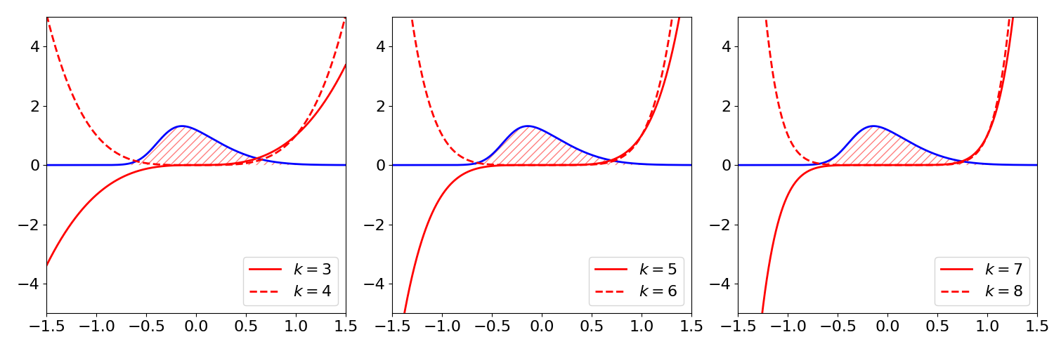
In that figure, I have plotted a skew normal distribution and overlaid the function $g(x; k) = x^k$ for odd and even powers of $k$. I have split the figure into three frames for legibility. Each function $g(x; k)$ represents how the $k$th moment (for $k \geq 3$) weights mass as that mass moves away from the zero mean of a centered distribution. We see that higher moments simply recapitulate the information captured by the third and fourth standardized moments. Thus, by convention, we only ever use skewness and kurtosis to describe a distribution because these are the lowest standardized moments that measure tailedness in their respective ways.

Moment-generating functions

While writing this blog post and trying to understand how moments quantify the location, scale, and shape of a distribution, I realized that a related theoretical idea made a lot more sense now: a random variable’s moment-generating function is an alternative specification of its distribution. Let me explain my intuition for why this feels almost obvious now.

Consider the moment-generating function (MGF) of a random variable $X$,

$M_X(t) = \mathbb{E}[e^{t X}], \quad t \in \mathbb{R}. \tag{31}$

To see why it is called a “moment-generating function”, note that

$\frac{d^k}{dt^k} M_X(t) = \mathbb{E}\left[\frac{d^k}{dt^k} e^{t X}\right] = \mathbb{E}[X^k e^{tX}] \tag{32}$

and therefore

$\frac{d^k}{dt^k} M_X(t) \Bigg|_{t=0} = \mathbb{E}[X^k]. \tag{33}$

In words, the $k$th derivative evaluated at the origin is the $k$th moment. This is nice. We can compute moments from the MGF by taking derivatives. This also means that the MGF’s Taylor series expansion,

$\mathbb{E}[e^{t X}] = \mathbb{E}\left[\sum_{k=0}^{\infty} \frac{1}{k!} t^k X^k \right] = \sum_{k=0}^{\infty} \frac{1}{k!} t^k \mathbb{E}[X^k], \tag{34}$

is really an infinite sum of weighted raw moments. MGFs are important for a lot of reasons, but perhaps the biggest is a uniqueness theorem:

Uniqueness theorem: Let $X$ and $Y$ be two random variables with cumulative distribution functions $F_X(x)$ and $F_Y(y)$. If the MGFs exist for $X$ and $Y$ and if $M_X(t) = M_Y(t)$ for all $t$ near $0$, then $F_X(z) = F_Y(z)$ for all $z \in \mathbb{R}$.

The big idea is that MGFs give us an another way to uniquely characterize the distribution of $X$. This is especially helpful since probability density functions and cumulative distribution functions can be hard to work with, and many times it is easier to shift a calculation to the realm of MGFs. See A5 for an example of a complicated calculation that is trivialized by MGFs.

This property, the fact that MGFs are unique and therefore an alternative way of specifying probability distributions, is what feels almost obvious now. Given what we know about moments and how they describe a distribution’s center of mass, spread, and relative and absolute size of the tails, it makes sense that a function that can generate all of the moments of a random variable is one way to fully describe that random variable. This is obviously not a proof. See Theorem $1.6$ in (Shao, 2003) for one. However, I suspect this intuition is how, if we were early probabilists, we might have hypothesized that such a result was provable.

Summary

Moments describe how the probability mass of a random variable is distributed. The zeroth moment, total mass, quantifies the fact that all distribution’s have a total mass of one. The first moment, the mean, specifies the distribution’s location, shifting the center of mass left or right. The second moment, variance, specifies the scale or spread; loosely speaking, flatter or more spread out distributions are “more random”. The third moment, skewness, quantifies the relative size of the two tails of a distribution; the sign indicates which tail is bigger and the magnitude indicates by how much. The fourth moment, kurtosis, captures the absolute size of the two tails. Higher standardized moments simply recapitulate the information in skewness and kurtosis; by convention, we ignore these in favor of the third and fourth standardized moments. Finally, moments are important theoretically because they provide an alternative way to fully and uniquely specify a probability distribution, a fact that is intuitive if you understand how moment’s quantify a distribution’s location, spread, and shape.

Acknowledgements

I thank Issa R, Michael D, Martin B, and Sam MK for catching various mistakes.

Appendix

A1. Skewness decomposition

By definition, skewness is

$\bar{m}_3 = \frac{m_3}{\sigma_3} \tag{A1}$

where $m_3$ is the third central moment and $\sigma_3$ is the standard deviation raised to the third power. We can decompose the numerator as

$\begin{aligned} m_3 &= \mathbb{E}[(X - \mu_x)^3] \\ &= \mathbb{E}[(X^2 - 2 X \mu_x + \mu_x^2)(X - \mu)] \\ &= \mathbb{E}[X^3 - 3X^2 \mu_x + 3 X \mu_x^2 - \mu_x^3] \\ &= \mathbb{E}[X^3 - 3 \mu_x (X^2 - X \mu_x) - \mu_x^3] \\ &\stackrel{\star}{=} \mathbb{E}[X^3] - 3 \mu_x \sigma_x^2 - \mu_x^3. \end{aligned} \tag{A2}$

In step $\star$, we use the fact that

$\mathbb{E}[X^2 - X \mu_x] = \mathbb{E}[X^2] - \mathbb{E}[X] \mu_x = \mathbb{E}[X^2] - \mathbb{E}[X]^2 = \sigma_x^2. \tag{A3}$

Therefore, we can express skewness entirely in terms of the first three raw moments:

$\bar{m}_3 = \frac{m_3}{\sigma_3} = \frac{\mathbb{E}[X^3] - 3 \mu_x \sigma_x^2 - \mu_x^3}{\sigma_3} = \frac{\mathbb{E}[X^3] - 3 \mathbb{E}[X] (\mathbb{E}[X^2] - \mathbb{E}[X]^2) - \mathbb{E}[X]^3}{(\mathbb{E}[X^2] - \mathbb{E}[X]^2)^{3/2}}. \tag{A4}$

A2. Root finding for Dagum distribution’s skewness parameter

import numpy as np
from   scipy.special import gamma
from   scipy.optimize import minimize


def pdf(x, beta, delta):
    """Compute probability density function of Dagum distribution. See:

    Dey 2017, "Dagum Distribution: Properties and Different Methods of 
    Estimation"
    """
    pos_x = x >  0
    neg_x = x <= 0
    pdf   = np.empty(x.size)
    A     = beta * delta * x[pos_x]**(-(delta+1))
    B     = (1 + x[pos_x]**(-delta))**(-(beta+1))
    pdf[pos_x] = A * B
    pdf[neg_x] = 0
    return pdf


def moment(k, beta, delta):
    """Compute k-th raw moment of Dagum distribution. See:

    Dey 2017, "Dagum Distribution: Properties and Different Methods of 
    Estimation"
    """
    A = gamma(1 - k/delta)
    B = gamma(beta + k/delta)
    C = gamma(beta)
    return (A * B) / C


def skewness(x, absolute=False):
    """Compute skewness using a decomposition of raw moments. If `absolute` is 
    `True`, return absolute value.
    """
    beta, delta = x
    EX1 = moment(1, beta, delta)
    EX2 = moment(2, beta, delta)
    EX3 = moment(3, beta, delta)
    var = EX2 - EX1**2
    mu3 = (EX3 - 3 * EX1 * var - EX1**3) / var**(3/2)
    if absolute:
        return abs(mu3)
    return mu3


SMALL = 1e-10
resp = minimize(
    fun=lambda x: skewness(x, absolute=True),
    x0=[0.5, 5],
    method='L-BFGS-B',
    bounds=[(SMALL, None), (SMALL, None)])
beta, delta = resp.x

print(f'Beta : {beta:.11f}')
print(f'Delta: {delta:.11f}')
print(f'Skew : {skewness([beta, delta]):.11f}')

A3. Kurtosis of any univariate normal is three

The density function of a univariate normal random variable with mean $\mu$ and variance $\sigma^2$ is

$f(x; \mu, \sigma^2) = \frac{1}{\sigma \sqrt{2 \pi}} \exp\Big\{-\frac{1}{2}\left(\frac{x - \mu}{\sigma}\right)^2\Big\}. \tag{A5}$

We can write the kurtosis as

$\begin{aligned} \mathbb{E}\left[ \left(\frac{X-\mu}{\sigma}\right)^4 \right] &= \int_{-\infty}^{\infty} \left(\frac{x-\mu}{\sigma}\right)^4 \frac{1}{\sigma \sqrt{2 \pi}} \exp\Big\{-\frac{1}{2}\left(\frac{x - \mu}{\sigma}\right)^2\Big\} \text{d}x \\ &= \frac{1}{\sigma \sqrt{2 \pi}} \int_{-\infty}^{\infty} \left(\frac{x-\mu}{\sigma}\right)^4 \exp\Big\{-\frac{1}{2}\left(\frac{x - \mu}{\sigma}\right)^2\Big\} \text{d}x \\ &= \frac{1}{\sqrt{2 \pi}} \int_{-\infty}^{\infty} a^4 \exp\Big\{-\frac{1}{2} a^2\Big\} \text{d}a. \end{aligned} \tag{A6}$

In the last step, we use integration by substitution where $a = (x-\mu)/\sigma$ and $\text{d}a = \text{d}x / \sigma$. This integral over an exponential function has an analytic solution:

$\int_{0}^{\infty} x^n e^{-b x^2} \text{d}x = \frac{(2k - 1)!!}{2^{k+1} a^k} \sqrt{\frac{\pi}{b}}, \qquad \text{$n = 2k$, $k$ integer, $b > 0$.} \tag{A7}$

For us, this means that

$\int_{0}^{\infty} a^4 \exp\Big\{-\frac{1}{2} a^2\Big\} \text{d}a = \frac{(2(2) - 1)!!}{2^{2+1} \frac{1}{2^2}} \sqrt{\frac{\pi}{\frac{1}{2}}} = \frac{3}{2} \sqrt{2 \pi}. \tag{A8}$

Since this is only half of the integral in $(\text{A}6)$, which we know is symmetric, the full integral is $3 \sqrt{2 \pi}$. The normalizer in $(\text{A}6)$ cancels, and we get

$\mathbb{E}\left[\left(\frac{X-\mu}{\sigma}\right)^4 \right] = \frac{1}{\sqrt{2 \pi}} \int_{-\infty}^{\infty} a^4 \exp\Big\{-\frac{1}{2} a^2\Big\} \text{d}a = 3. \tag{A9}$

A4. Mean and standard deviation of standard scores

The mean and standard deviation of the standard score ($z$-score) are zero and one respectively. Let $X$ be a random variable with mean $\mu_x$ and standard deviation $\sigma_x$. The standard score is defined as

$z = \frac{x - \mu_x}{\sigma_x}. \tag{A10}$

The mean of the standard scores is then

$\mu_z = \frac{1}{N} \sum_{n=1}^{N} z_n = \frac{1}{N} \sum_{n=1}^{N} \frac{x_n - \mu_x}{\sigma_x} = 0. \tag{A11}$

The last equality holds because

$\sum_{n=1}^{N} (x_n - \mu_x) = \sum_{n=1}^{N} x_n - \sum_{n=1}^{N} \mu_x = N \mu_x - N \mu_x. \tag{A12}$

The standard deviation of the standard scores is then

$\begin{aligned} \sigma_z &= \frac{1}{N} \sum_{n=1}^{N} (z_n - \mu_z)^2 \\ &= \frac{1}{N} \sum_{n=1}^{N} z_n^2 \\ &= \frac{1}{N} \sum_{n=1}^{N} \left( \frac{x_n - \mu_x}{\sigma_x} \right)^2 \\ &= \frac{1}{\sigma_x^2} \underbrace{\frac{1}{N} \sum_{n=1}^{N} ( x_n - \mu_x)^2}_{\sigma_x^2} \\ &= 1. \end{aligned} \tag{A13}$

A5. Convolution of independent gammas random variables

Here is an example of a calculation that is made surprisingly easy by working with MGFs rather than distribution functions. Let $X_1 \sim \text{Gamma}(\alpha_1, \beta)$ and $X_2 \sim \text{Gamma}(\alpha_2, \beta)$ be independent random variables. What is the distribution of $Y = X_1 + X_2$? Well, the moment generating function of $X_1 \sim \text{Gamma}(\alpha_1, \beta)$ is

$M_{X_1}(t) = \mathbb{E}[e^{tX_1}] = \Bigg(\frac{\beta}{\beta - t}\Bigg)^{\alpha_1}. \tag{A14}$

Since $X_1$ and $X_2$ are independent, we know the MGF of $Y = X_1 + X_2$ decomposes as

$M_Y(t) = M_{X_1}(t) M_{X_2}(t). \tag{A15}$

The fact that summing independent random variables reduces to multiplying their MGFs is an important property of MGFs. See (Shao, 2003), around equation $1.58$, for a discussion. Thus, the MGF of $Y$ must be

$\Bigg(\frac{\beta}{\beta - t}\Bigg)^{\alpha_1} \Bigg(\frac{\beta}{\beta - t}\Bigg)^{\alpha_2} = \Bigg(\frac{\beta}{\beta - t}\Bigg)^{\alpha_1 + \alpha_2}, \tag{A16}$

which means that $Y \sim \text{Gamma}(\alpha_1 + \alpha_2, \beta)$. I’m not sure how I would have approached this problem using the cumulative distribution or probability density functions.

To derive the MGF of the gamma distribution ourselves, note that

$\begin{aligned} M_{X}(t) &= \mathbb{E}[e^{tX}] \\ &= \int_{0}^{\infty} e^{tx} \frac{\beta^{\alpha}}{\Gamma(\alpha)} x^{\alpha - 1} e^{-\beta x} \text{d}x \\ &= \frac{\beta^{\alpha}}{\Gamma(\alpha)} \int_{0}^{\infty} e^{tx} x^{\alpha - 1} e^{-\beta x} \text{d}x \\ &= \frac{\beta^{\alpha}}{\Gamma(\alpha)} \int_{0}^{\infty} x^{\alpha - 1} e^{-x(\beta - t)} \text{d}x \\ &\stackrel{\star}{=} \frac{\beta^{\alpha}}{\Gamma(\alpha)} \frac{\Gamma(\alpha)}{(\beta - t)^{\alpha}} \\ &= \Bigg(\frac{\beta}{\beta - t}\Bigg)^{\alpha}. \end{aligned} \tag{A17}$

Step $\star$ holds because

$\int_{0}^{\infty} x^{a} e^{-bx} = \frac{\Gamma(a+1)}{b^{a+1}}. \tag{A18}$