Bayesian Linear Regression

A Bayesian approach

In my first post on linear models, I discussed ordinary least squares (OLS) regression. OLS is simple, interpretable, and well-understood. The parameter estimate which minimizes the sum of squared residuals is also the maximum likelihood estimate (MLE) under a probabilistic interpretation of the model. MLEs are theoretically well-understood. For example, MLEs are asymptotically normal and many achieve the Cramér–Rao lower bound, meaning they have minimum possible variance in the class of unbiased estimators. However, OLS can overfit, which I discussed in my second post on linear models. We can see this by looking at the model for linear regression,

$y_n = \boldsymbol{\beta}^{\top} \mathbf{x}_n + \varepsilon_n. \tag{1}$

Above, $\mathbf{x}_n$ is the $n$th data point, a $P$-vector of predictors; $y_n$ is a scalar response; $\boldsymbol{\beta}$ is a $P$-vector of coefficients; and $\varepsilon_n \sim \mathcal{N}(0, \sigma^2)$ is unobserved noise. Notice that even if a true coefficient value (a component of $\boldsymbol{\beta}$) is zero, the learned coefficient will not be because of the noise term $\varepsilon_n$.

Another way to see this is to think about the probabilistic interpretation of $(1)$,

$y_n \mid \boldsymbol{\beta}, \sigma^2 \sim \mathcal{N}(y_n \mid \boldsymbol{\beta}^{\top} \mathbf{x}_n, \sigma^2). \tag{2}$

Here, $y_n$ is a random variable with mean $\boldsymbol{\beta}^{\top} \mathbf{x}_n$ and variance $\sigma^2$. Even if the true mean is a $P$-vector of zeros, $y_n$ is a random quantity since $\sigma^2$ is nonzero.

A Bayesian approach to tackling this problem is to use priors. A prior is a distribution on a parameter. To give some intuition for why this might be useful, consider the task of inferring the bias of a coin. If you could flip the coin an infinite number of times, inferring its bias would be easy by the law of large numbers. However, what if you could only flip the coin a handful of times? Would you guess that a coin is biased if you saw three heads in three flips, an event that happens one out of eight times with unbiased coins? The MLE would overfit these data, inferring a coin bias of $p = 1$. A Bayesian approach avoids overfitting by quantifying our prior knowledge that most coins are unbiased, that the prior on the bias parameter is peaked around one-half. The data must overwhelm this prior belief about coins.

In Bayesian linear regression, we place a prior on $\boldsymbol{\beta}$ that is a zero-centered and symmetric distribution. In my mind, this prior on $\boldsymbol{\beta}$ is almost like a null hypothesis; it is the modeling assumption equivalent that there is no relationship between $\mathbf{x}_n$ and $y_n$. Recall that a small coefficient $\beta_p$ indicates that the marginal effect of the $p$th predictor is negligible. It is up to the data to prove this belief wrong.

Example

Bayesian inference amounts to inferring a posterior distribution $p(\boldsymbol{\beta} \mid \mathbf{X}, \mathbf{y})$ where I use $\mathbf{X}$ to denote an $N \times P$ matrix of predictors and $\mathbf{y}$ to denote an $N$-vector of scalar responses. The idea is to use Bayes’ formula to compute this,

$\overbrace{\phantom{\Big[} p(\boldsymbol{\beta} \mid \mathbf{X}, \mathbf{y}) }^{\text{posterior}} \propto \overbrace{\phantom{\Big[} p(\mathbf{X}, \mathbf{y} \mid \boldsymbol{\beta}) }^{\text{likelihood}} \overbrace{\phantom{\Big[} p(\boldsymbol{\beta}) }^{\text{prior}}. \tag{3}$

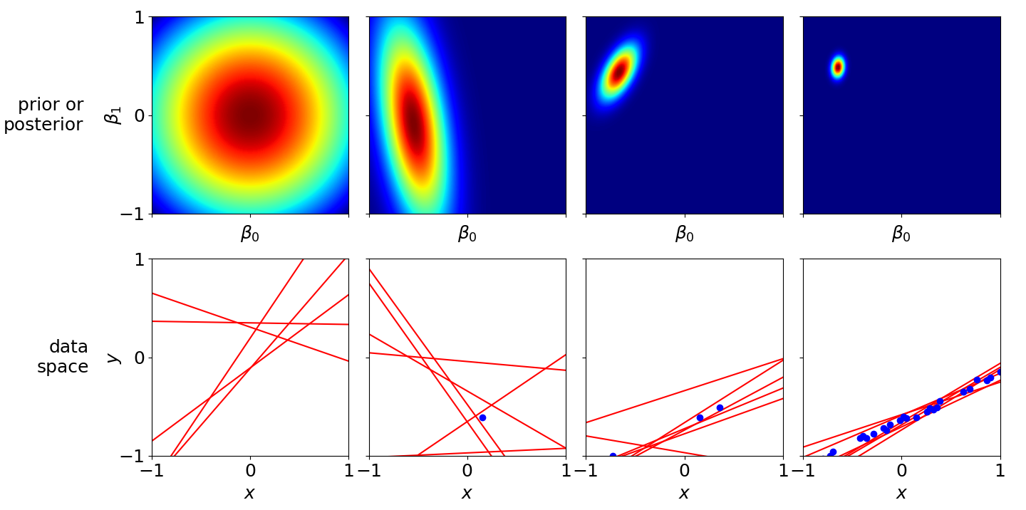
Performing exact Bayesian inference can be extremely tedious because it involves lots of calculations to ensure the inferred distributions are tractable. However, before getting into the weeds, let’s look at a motivating example. (Bishop, 2006) has a famous figure (his Figure $3.7$) explaining Bayesian linear regression, and I’ve reproduced a version of that figure with my own implementation of Bayesian linear regression (my Figure $1$). It is really worth spending time on this figure because it captures some key ideas in Bayesian inference.

Figure 1. Bayesian linear regression using the hierarchical prior in $(5)$. The top row visualizes the prior (top left frame) and posterior (top right three frames) distributions on the parameter $\boldsymbol{\beta}$ with an increasing (left-to-right) number of observations. The bottom row visualizes six draws of $\boldsymbol{\beta}$ from each frame's respective distribution (the frame above). The data is generated using true bias and slope parameters $\boldsymbol{\beta}_{\texttt{true}} = [0.5, -0.7]^{\top}$. See this GitHub repo for code to reproduce the figures in this post.

The true generative model is scalar data with a bias term,

$y_n = 0.5 x_n - 0.7 \tag{4}$

where $\beta_1 = 0.5$ and the bias is $\beta_0 = -0.7$. This allows us to plot the coefficients in two-dimensions (top row) while visualizing the inferred hyperplanes in two-dimensions as well (bottom row). In the first column, the model has seen no data. The prior places high and equal probability on both $\beta_0$ and $\beta_1$ being zero. Six random samples of the vector $\boldsymbol{\beta} = [\beta_0, \beta_1]^{\top}$ are shown in the bottom row; these are draws from our prior distribution on $\boldsymbol{\beta}$. In subsequent columns, the model is fit to more data. As we can see, with more data the model’s inferred posterior variance decreases, and the realizations of $\boldsymbol{\beta}$ from the posterior become more constrained.

Tractability through conjugacy

In principle, we can use any prior on our parameters that we would like. However, the functional form of most priors, when multiplied by the functional form of the likelihood in $(3)$, results in an posterior with no closed-form solution. It might also be tricky to draw samples or compute moments. In these cases, we would resort to approximate Bayesian inference techniques such as Monte Carlo methods or variational inference. Thus, certain priors are mathematically convenient because they result in posteriors with tractable, well-known densities. This typically occurs when the prior is conjugate, meaning that the prior and posterior share the same functional form. In Bayesian linear regression, a common conjugate prior on the two parameters $\boldsymbol{\beta}$ and $\sigma^2$ is a normal–inverse–gamma distribution,

$\begin{aligned} p(\boldsymbol{\beta}, \sigma^2) &= p(\boldsymbol{\beta} \mid \sigma^2) p(\sigma^2) \\ &\text{where} \\ \boldsymbol{\beta} \mid \sigma^2 &\sim \mathcal{N}_P(\mathbf{0}, \sigma^2 \boldsymbol{\Lambda}_0^{-1}) \\ \sigma^2 &\sim \text{InvGamma}(a_0, b_0). \end{aligned} \tag{5}$

Since this model is conjugate, we know that the derived posterior must be a normal–inverse–gamma distribution, which we will show. Note that in this model, we learn both $\boldsymbol{\beta}$ and variance of the noise $\sigma^2$ by placing a conditional prior on $\boldsymbol{\beta}$. These kinds of priors are sometimes called hierarchical. Other conjugate priors might assume either $\boldsymbol{\beta}$ or $\sigma^2$ are known.

Conjugate priors often lend themselves to other tractable distributions of interest. For example, the model evidence or marginal likelihood is defined as the probability of an observation after integrating out the model’s parameters,

$p(\mathbf{y} \mid \boldsymbol{\alpha}) = \int\!\!\!\int p(\mathbf{y} \mid \mathbf{X}, \boldsymbol{\beta}, \sigma^2) p(\boldsymbol{\beta}, \sigma^2 \mid \boldsymbol{\alpha}) \,\text{d}^P\boldsymbol{\beta} \,\text{d}\sigma^2. \tag{6}$

In the case of $(5)$, $\boldsymbol{\alpha} = \{a_0, b_0\}$. As we will see, we can easily compute $(6)$ because we know the normalizing quantities of the normal and inverse–gamma distributions and can therefore compute the integrals in closed-form.

Following the same logic as above, we can also compute the predictive or posterior predictive distribution or the probability of an unseen observation given observed data,

$p(\hat{\mathbf{y}} \mid \mathbf{y}) = \int\!\!\!\int \overbrace{p(\hat{\mathbf{y}} \mid \mathbf{\hat{X}}, \boldsymbol{\beta}, \sigma^2)}^{\text{model}} p(\boldsymbol{\beta} \mid \mathbf{X}, \mathbf{y}, \sigma^2) p(\sigma^2 \mid \mathbf{X}, \mathbf{y}) \text{d}^P\boldsymbol{\beta} \text{d}\sigma^2. \tag{7}$

Note that in the term labeled “model”, we condition on the new observations’ predictors. We will see that $p(\mathbf{\hat{y}} \mid \mathbf{y})$ is a multivariate t-distribution under $(5)$. To perform prediction, we take the mean of this distribution. Its variance can be interpreted as how certain the model is of that prediction. Again, this is relatively straightforward to compute because we know the normalizing quantities of the distributions with which we are working.

Now that we have some intuition for the benefits of Bayesian linear regression and tractable conjugate priors, let’s fully derive the posterior, marginal likelihood, and predictive distributions of the model under $(5)$. We’ll look at examples along the way to provide some intuition.

Posterior

We want to show that the normally distributed likelihood can be decomposed into a functional form that looks a lot like a normal–inverse–gamma density. Since we have a normal–inverse–gamma prior, this allows us to consolidate “like terms” to generate a normal–inverse–gamma posterior.

Let’s get into the weeds. Respectively, our likelihood, conditional prior on $\boldsymbol{\beta}$, and prior on $\sigma^2$ are

$\begin{aligned} p(\mathbf{y} \mid \mathbf{X}, \boldsymbol{\beta}, \sigma^2) &= (2 \pi \sigma^2)^{-N/2} \exp\!\Big(\!-\frac{1}{2 \sigma^2} (\mathbf{y} - \mathbf{X} \boldsymbol{\beta})^{\top} (\mathbf{y} - \mathbf{X} \boldsymbol{\beta}) \Big) \\ p(\boldsymbol{\beta} \mid \sigma^2) &= (2 \pi \sigma^2)^{-P/2} \big|\boldsymbol{\Lambda}_0 \big|^{1/2} \exp\Big(\!-\frac{1}{2\sigma^2} (\boldsymbol{\beta} - \boldsymbol{\mu}_0)^{\top} \boldsymbol{\Lambda}_0 (\boldsymbol{\beta} - \boldsymbol{\mu}_0) \Big) \\ p(\sigma^2) &= \frac{b_0^{a_0}}{\Gamma(a_0)} (\sigma^2)^{-(a_0 + 1)} \exp(-b_0 / \sigma^2). \end{aligned} \tag{8}$

See (A1) and (A2) for detailed steps arriving at these particular formulations and (A3) for my formulation of the inverse–gamma distribution (it has multiple parameterizations). Now notice that we can decompose the likelihood’s Gaussian kernel and combine it with the prior’s kernel in the following way:

$\begin{aligned} &(\mathbf{y} - \mathbf{X}\boldsymbol{\beta})^{\top} (\mathbf{y} - \mathbf{X}\boldsymbol{\beta}) + (\boldsymbol{\beta} - \boldsymbol{\mu}_0)^{\top} \boldsymbol{\Lambda}_0 (\boldsymbol{\beta} - \boldsymbol{\mu}_0) \\ &= (\mathbf{y} - \mathbf{X} \boldsymbol{\hat{\beta}})^{\top}(\mathbf{y} - \mathbf{X} \boldsymbol{\hat{\beta}}) + (\boldsymbol{\hat{\beta}} - \boldsymbol{\beta})^{\top} \mathbf{X}^{\top} \mathbf{X} (\boldsymbol{\hat{\beta}} - \boldsymbol{\beta}) + (\boldsymbol{\beta} - \boldsymbol{\mu}_0)^{\top} \boldsymbol{\Lambda}_0 (\boldsymbol{\beta} - \boldsymbol{\mu}_0) \\ &= \mathbf{y}^{\top} \mathbf{y} + \boldsymbol{\mu}_0 \boldsymbol{\Lambda}_0 \boldsymbol{\mu}_0 - \boldsymbol{\mu}_N^{\top} \boldsymbol{\Lambda}_N \boldsymbol{\mu}_N + (\boldsymbol{\beta} - \boldsymbol{\mu}_N)^{\top} \boldsymbol{\Lambda}_N (\boldsymbol{\beta} - \boldsymbol{\mu}_N). \end{aligned} \tag{9}$

where $\boldsymbol{\mu}_N$ and $\boldsymbol{\Lambda}_N$ are defined as

$\begin{aligned} \boldsymbol{\Lambda}_N &= \mathbf{X}^{\top} \mathbf{X} + \boldsymbol{\Lambda}_0 \\ \boldsymbol{\mu}_N &= \boldsymbol{\Lambda}_N^{-1} (\boldsymbol{\mu}_0^{\top} \boldsymbol{\Lambda}_0 + \mathbf{X}^{\top} \mathbf{y}). \end{aligned} \tag{10}$

(Note: I use “kernel” to refer to a density in which any constants or terms that are not variables of interest are omitted.) Currently, I don’t think there’s no easy way to intuit $(9)$ and $(10)$. It requires a lot of algebra which I’ve included in (A4) and (A5). I don’t want to clutter the main line of thinking with those derivations, but I do encourage you to read those appendices carefully. That said, the main idea is that we consolidated terms to make a Gaussian kernel that is quadratic in $\boldsymbol{\beta}$ and moved the remaining terms into an inverse–gamma density, thus generating a posterior that is proportional to a normal–inverse–gamma density.

Now our posterior can be written as

$\begin{aligned} p(\mathbf{y} \mid \mathbf{X}, \boldsymbol{\beta}, \sigma^2) &\propto (2 \pi \sigma^2)^{-P/2} \big|\boldsymbol{\Lambda}_0 \big|^{1/2} \exp\Big(-\frac{1}{2\sigma^2}\Big[(\boldsymbol{\beta} - \boldsymbol{\mu}_N)^{\top} \boldsymbol{\Lambda}_N (\boldsymbol{\beta} - \boldsymbol{\mu}_N)\Big]\Big) \\ &\;\;\;\; (2 \pi \sigma^2)^{-N/2} \exp\Big(-\frac{1}{2 \sigma^2}\Big[ \mathbf{y}^{\top} \mathbf{y} + \boldsymbol{\mu}_0 \boldsymbol{\Lambda}_0 \boldsymbol{\mu}_0 - \boldsymbol{\mu}_N^{\top} \boldsymbol{\Lambda}_N \boldsymbol{\mu}_N \Big]\Big) \\ &\;\;\;\; \frac{b_0^{a_0}}{\Gamma(a_0)} (\sigma^2)^{-(a_0 + 1)} \exp(-b_0 / \sigma^2). \end{aligned} \tag{11}$

We can see that we have a $P$-variate normal distribution on the first line. If we ignore $(2 \pi)^{-N/2}$ and inverse–gamma prior normalizer, we can combine the bottom two lines to be proportional to an inverse–gamma distribution,

$(\sigma^2)^{-(a_0 + N/2 + 1)} \exp\Big(-\frac{1}{\sigma^2}\Big[ b_0 + \frac{1}{2} \Big\{\mathbf{y}^{\top} \mathbf{y} + \boldsymbol{\mu}_0 \boldsymbol{\Lambda}_0 \boldsymbol{\mu}_0 - \boldsymbol{\mu}_N^{\top} \boldsymbol{\Lambda}_N \boldsymbol{\mu}_N \Big\}\Big]\Big). \tag{12}$

Now define $a_N$ and $b_N$ as

$\begin{aligned} a_N &= a_0 + \frac{N}{2} \\ b_N &= b_0 + \frac{1}{2}(\mathbf{y}^{\top} \mathbf{y} + \boldsymbol{\mu}_0 \boldsymbol{\Lambda}_0 \boldsymbol{\mu}_0 - \boldsymbol{\mu}_N^{\top} \boldsymbol{\Lambda}_N \boldsymbol{\mu}_N). \end{aligned} \tag{13}$

In summary, we can write our posterior as

$\begin{aligned} p(\boldsymbol{\beta}, \sigma^2 \mid \mathbf{X}, \mathbf{y}) &\propto p(\boldsymbol{\beta} \mid \mathbf{X}, \mathbf{y}, \sigma^2) p(\sigma^2 \mid \mathbf{X}, \mathbf{y}) \\ &\!\!\!\!\text{where} \\ \boldsymbol{\beta} \mid \mathbf{X}, \mathbf{y}, \sigma^2 &\sim \mathcal{N}_P(\boldsymbol{\mu}_N, \sigma^2 \boldsymbol{\Lambda}_N^{-1}) \\ \sigma^2 \mid \mathbf{y}, \mathbf{X} &\sim \text{InvGamma}(a_N, b_N). \end{aligned} \tag{14}$

Of course, we have ignored constants and the normalizing evidence because we only care about the shape of the posterior with respect to the model parameters.

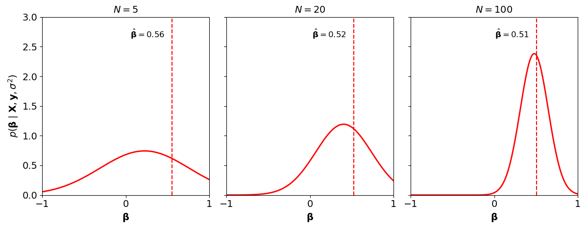
Figure 2. The OLS point estimate of $\boldsymbol{\beta}$ (dashed red line) and Bayesian linear regression's posterior distribution (solid red line) fit to an increasing number of observations.

To get some intuition for what the posterior represents, consider Figure $2$, which compares OLS with Baysesian linear regression on an increasing number of data points. OLS has no notion of uncertainty about its point estimate of $\boldsymbol{\beta}$. Bayesian linear regression does; and being regularized by its prior, it requires more data to become more certain about the inferred $\boldsymbol{\beta}$. In many models, the MLE and posterior mode are equivalent in the limit of infinite data.

Marginal likelihood

To compute the model evidence or marginal likelihood, we need to compute the following integral,

$p(\mathbf{y} \mid \boldsymbol{\alpha}) = \int\!\!\!\int p(\mathbf{y} \mid \mathbf{X}, \boldsymbol{\beta}, \sigma^2) p(\boldsymbol{\beta}, \sigma^2 \mid \boldsymbol{\alpha}) \,\text{d}^P\boldsymbol{\beta} \,\text{d}\sigma^2 \tag{15}$

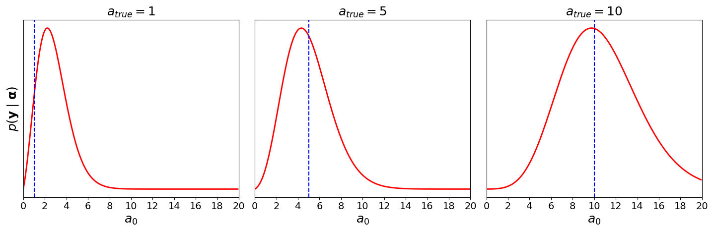
where $\boldsymbol{\alpha} = \{a_0, b_0\}$. Note that the integral is high-dimensional since we’re integrating over two variables, one of which is itself high-dimensional. To give some intuition for what this means, consider Figure $3$. Each subplot represents the Bayesian linear regression model in $(5)$ fit with different initial values $a_0$. The model was fit to synthetic data that was generated using $a_{\texttt{true}}$ as the true hyperprior for the inverse–gamma prior on $\sigma^2$. The other parameter, $b_0$, was fixed. We can see that the model evidence is useful for model comparisons; it tells us how well a particular model—a point on the curve in Figure $3$—does relative to other models.

Figure 3. Bayesian linear regression fit with different initial values of $a_0$. In each frame, the data was generated using $a_{\texttt{true}}$ (dashed blue line) as the true hyperprior for the inverse–gamma prior.

Computing $(15)$ is easier than it looks. First, we can write the integrated terms (the joint) in $(15)$ using the definitions in $(10)$ and $(13)$,

$\begin{aligned} p(\mathbf{y}, \boldsymbol{\beta}, \sigma^2) &= (2 \pi \sigma^2)^{-P/2} \big|\boldsymbol{\Lambda}_0 \big|^{1/2} \exp\!\Big(\!-\frac{1}{2\sigma^2}\Big[(\boldsymbol{\beta} - \boldsymbol{\mu}_N)^{\top} \boldsymbol{\Lambda}_N (\boldsymbol{\beta} - \boldsymbol{\mu}_N)\Big]\Big) \\ &\;\;\;\; (\sigma^2)^{-(a_N + 1)} \exp\!\Big(\!-\frac{b_N}{\sigma^2}\Big) \\ &\;\;\;\; (2 \pi)^{-N/2} \frac{b_0^{a_0}}{\Gamma(a_0)}. \end{aligned} \tag{16}$

Now notice that since the integral over $\boldsymbol{\beta}$ is only over the Gaussian kernel. Since we know the normalizer for the multivariate normal, we can compute this immediately:

$(2\pi\sigma^2)^{P/2} \big| \boldsymbol{\Lambda}_N\big|^{-1/2} = \int \exp\Big( -\frac{1}{2} (\boldsymbol{\beta} - \boldsymbol{\mu}_N)^{\top} \Big[ \frac{1}{\sigma^2} \boldsymbol{\Lambda}_N \Big] (\boldsymbol{\beta} - \boldsymbol{\mu}_N) \Big) \text{d}^P \boldsymbol{\beta} \tag{17}$

See (A6) for details. We can see that $(2\pi\sigma^2)^{P/2}$ will cancel with the other normalizing constant, reducing the first line in $(16)$ to

$\sqrt{\frac{|\boldsymbol{\Lambda}_0 |}{|\boldsymbol{\Lambda}_N |}}. \tag{18}$

We can compute the second integral (over the second line of $16$) because we know the normalizing constant of the gamma kernel,

$\frac{\Gamma(a_N)}{b_N^{a_N}} = \int (\sigma^2)^{-(a_N + 1)} \exp\!\Big(\!-\frac{b_N}{\sigma^2}\Big) \text{d}\sigma^2. \tag{19}$

Putting it all together, we get

$p(\mathbf{y}) = \frac{1}{(2 \pi)^{N/2}} \sqrt{\frac{|\boldsymbol{\Lambda}_0 |}{|\boldsymbol{\Lambda}_N |}} \cdot \frac{b_0^{a_0}}{b_N^{a_N}} \cdot \frac{\Gamma(a_N)}{\Gamma(a_0)}. \tag{20}$

While this was a bit tedious to write out, it demonstrates the utility of conjugacy and staying within families of well-understood distributions. In general, integrating $(15)$ exactly is intractable, but we handled it easily and without any calculus.

Posterior predictive

In the last two sections, we saw two benefits to a Bayesian approach to linear regression. First, rather than inferring a point estimate for $\boldsymbol{\beta}$, we inferred a distribution that quantifies the model’s uncertainty about its estimate. Second, we saw that we can perform model criticism using the marginal likelihood or model evidence. This gives us a principled way to compare models. However, much of the time we are most interested in prediction. Given the data we have seen so far and our parameter estimates, what is our predicted value for a new data point?

We might be tempted to just use the mean of the posterior over $\boldsymbol{\beta}$, $\boldsymbol{\mu}_N$, as our predicted hyperplane. However, we can do something more principled than this using the predictive distribution, sometimes called the posterior predictive distribution. This is the distribution over unobserved data $\mathbf{\hat{y}}$, which we can represent by integrating out the model parameters. Let’s rewrite $(7)$ as

$p(\hat{\mathbf{y}} \mid \mathbf{y}) = \int p(\sigma^2 \mid \mathbf{X}, \mathbf{y}) \Big[ \int \overbrace{p(\hat{\mathbf{y}} \mid \hat{\mathbf{X}}, \boldsymbol{\beta}, \sigma^2)}^{\text{model}} p(\boldsymbol{\beta} \mid \mathbf{X}, \mathbf{y}, \sigma^2) \text{d}^P \boldsymbol{\beta} \Big] \text{d}\sigma^2. \tag{21}$

I think of $(21)$ as answering the question, “What is the distribution over unseen data given all possible parameter estimates that we could have inferred from seen data?” The integration weights the model’s prediction of new data by the posterior’s parameter estimates from observed data. I believe this really captures what most researchers mean when they say that Bayesian methods “quantify uncertainty”. Our model explicitly encodes how uncertain it is about its parameter estimates using the posterior distribution, and the posterior predictive distribution uses that uncertainty to weight the probability of new observations.

Once again, we can calculate this high-dimensional integral without calculus because of conjugacy. First, the two terms in the integral over $\boldsymbol{\beta}$ are normally distributed,

$\begin{aligned} p(\hat{\mathbf{y}} \mid \mathbf{\hat{X}}, \boldsymbol{\beta}, \sigma^2) &= \mathcal{N}(\hat{\mathbf{y}} \mid \mathbf{\hat{X}}\boldsymbol{\beta}, \sigma^2 \mathbf{I}) \\ p(\boldsymbol{\beta} \mid \mathbf{X}, \mathbf{y}, \sigma^2) &= \mathcal{N}(\boldsymbol{\beta} \mid \boldsymbol{\mu}_N, \sigma^2 \boldsymbol{\Lambda}_N^{-1}). \end{aligned} \tag{22}$

We can use properties of normally distributed random variables to compute this integral. See (Bishop, 2006), equations $2.113$, $2.114$, and $2.115$:

$p(\hat{\mathbf{y}} \mid \hat{\mathbf{X}}, \mathbf{y}, \sigma^2) = \mathcal{N}_M( \hat{\mathbf{y}} \mid \hat{\mathbf{X}} \boldsymbol{\mu}_N, \sigma^2 \mathbf{I} + \hat{\mathbf{X}} [\sigma^2 \boldsymbol{\Lambda}_N] \hat{\mathbf{X}}^{\top} ). \tag{23}$

Just to be clear, this is an $M$-variate distribution where $M$ is the number of testing samples in $\mathbf{\hat{X}}$. Thus, the posterior predictive can be written as

$p(\hat{\mathbf{y}} \mid \mathbf{y}) = \int p(\hat{\mathbf{y}} \mid \hat{\mathbf{X}}, \mathbf{y}, \sigma^2) p(\sigma^2 \mid \mathbf{X}, \mathbf{y}) \text{d}\sigma^2. \tag{24}$

Computing the integral over $\sigma^2$ and simplifying is straightforward—we use the same tricks as above—, but it is rather tedious. Rather than disrupt the main line of thinking, I have included that derivation in (A7). The upshot is that the posterior predictive is an $M$-variate t-distribution,

$p(\hat{\mathbf{y}} \mid \mathbf{y}) = \frac{\Gamma(\frac{\nu + M}{2})}{\Gamma(\nu/2) \nu^{M/2} \pi^{M/2} |\boldsymbol{\Sigma}|^{1/2}} \Big[1 + \frac{1}{\nu}(\mathbf{\hat{y}} - \mathbf{m}) \boldsymbol{\Sigma}^{-1}(\mathbf{\hat{y}} - \mathbf{m})\Big]^{-(\frac{\nu + M}{2})} \tag{25}$

with mean $\mathbf{m}$, shape matrix $\boldsymbol{\Sigma}$, and degrees of freedom $\nu$:

$\begin{aligned} \mathbf{m} &= \hat{\mathbf{X}}\boldsymbol{\mu}_N \\ \boldsymbol{\Sigma} &= \frac{b_N}{a_N} \mathbf{V} = \frac{b_N}{a_N} (\mathbf{I} + \hat{\mathbf{X}} \boldsymbol{\Lambda}_N \hat{\mathbf{X}}^{\top}) \\ \nu &= 2 a_N. \end{aligned} \tag{26}$

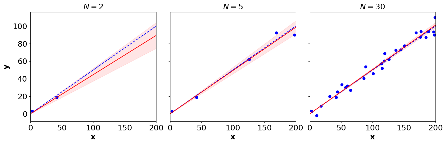
Now let’s look at why the posterior predictive is useful. As we just saw, under the model in $(5)$, the predictive $p(\mathbf{\hat{y}} \mid \mathbf{y})$ is a multivariate t-distribution. This means we have closed-form estimates of our predictive distribution’s moments. To understand what this means, consider Figure $4$.

Figure 4. The posterior predictive distribution's mean (solid red line) and two standard deviations from the mean (pink region) after fitting the model in $(5)$ to $N$ data points. The true data generating function is denoted with dashed blue lines.

In each frame, Bayesian linear regression is fit to $N$ data points, and then the mean and two standard deviations around the mean of the posterior predictive distribution are plotted. We can see that the model is less certain in its predictions in regions where it has seen less data or less consistent data. This is a simplified version of Bishop’s Figure $3.8$ using the model in $(5)$ rather than Gaussian basis functions. In other words, uncertainty about $\boldsymbol{\beta}$ is combined with the underlying probabilistic model of the data to generating principled predictions about what new data is plausible.

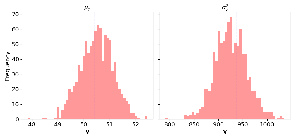
Figure 5. Posterior predictive checks of the mean (left) and variance (right) of the model in $(5)$. The finite sample mean and variance are plotted in blue dashed lines. The histograms are binned over one thousand statistics computed from finite samples from the posterior predictive distribution.

Another use of the posterior predictive is performing posterior predictive checks (Box, 1980). George Box is famous for saying, “All models are wrong, but some are useful.” I think of posterior predictive checks as measuring how good of an approximation of reality our model really is. The basic idea is to draw samples from the posterior predictive distribution and then compare them to our observations. For example, consider Figure $5$. Given one hundred observations $\mathbf{y} = [y_1, \dots y_{100}]^{\top}$, we fit a model. Then we draw a thousand random variables, $\mathbf{\hat{y}}_1, \dots, \mathbf{\hat{y}}_{1000}$, from the posterior predictive distribution. To be clear, this posterior predictive check uses the training data twice. Thus, each $\mathbf{\hat{y}}_i$ is a draw from a $100$-variate t-distribution and is therefore itself a $100$-dimensional vector. (My understanding is that there is some debate about this (see here for more), but I don’t think it is critical for the main line of thinking. One could easily hold out $M$ observations and sample $M$-dimensional $\mathbf{\hat{y}}_i$ instead.) Next, for each $\mathbf{\hat{y}}_i$, we compute the sample mean and sample variance. Finally, we compare a histogram of these means and variances to the observed mean and variance. If our model is a good approximation of reality, these histograms will be tightly centered around the observations.

Conclusion

As this post has probably made clear, exact Bayesian inference is rather tedious. Even when working with simple and well-understood distributions, we had to churn through a lot of derivations using linear algebra and probability to arrive at tractable distributions. However, the Bayesian approach to linear regression is well-motivated. Rather than inferring a point estimate of our parameter $\boldsymbol{\beta}$, we infer a distribution over it. The prior acts as a regularizer against overfitting, and the posterior quantifies how certain the model is in its parameter estimates. Furthermore, this approach gives us principled methods for performing model criticism and prediction using the marginal likelihood and posterior predictive distributions.

Acknowledgements

I thank Mathijs de Jong for correcting a mistake in derivation A4.

Appendix

See this GitHub repo for code to reproduce the figures in this post.

A1. Density for $\mathcal{N}(\boldsymbol{\beta}^{\top} \mathbf{X}, \sigma^2 \mathbf{I})$

If $\mathbf{y} \sim \mathcal{N}(\boldsymbol{\beta}^{\top} \mathbf{X}, \sigma^2 \mathbf{I})$, then its density is

$p(\mathbf{y} \mid \mathbf{X}, \boldsymbol{\beta}, \sigma^2) = \frac{1}{\sqrt{(2 \pi)^N |\sigma^2 \mathbf{I}|}} \exp\Big(-\frac{1}{2}(\mathbf{y} - \boldsymbol{\beta}^{\top} \mathbf{X})^{\top} [\sigma^2 \mathbf{I}]^{-1}(\mathbf{y} - \boldsymbol{\beta}^{\top} \mathbf{X})\Big) \tag{A1.1}$

The determinant of a diagonal matrix is the product of its diagonal elements, and therefore

$|\sigma^2 \mathbf{I}| = (\sigma^2)^N. \tag{A1.2}$

Furthermore, the inverse of a diagonal matrix is just the inverse of each diagonal element or

$[\sigma^2 \mathbf{I}]^{-1} = \begin{bmatrix} 1 / \sigma^2 & & \\ & \ddots & \\ & & 1 / \sigma^2 \end{bmatrix}. \tag{A1.3}$

Finally, a vector times a diagonal matrix is equivalent to element-wise multiplication of the vector with the diagonal elements. Therefore, we can write

$-\frac{1}{2} (\mathbf{y} - \boldsymbol{\beta}^{\top} \mathbf{X})^{\top} [\sigma^2 \mathbf{I}]^{-1}(\mathbf{y} - \boldsymbol{\beta}^{\top} \mathbf{X}) = -\frac{1}{2 \sigma^2} (\mathbf{y} - \boldsymbol{\beta}^{\top} \mathbf{X})^{\top} (\mathbf{y} - \boldsymbol{\beta}^{\top} \mathbf{X}). \tag{A1.4}$

Putting it all together, we can write the density as

$p(\mathbf{y} \mid \mathbf{X}, \boldsymbol{\beta}, \sigma^2) = (2 \pi \sigma^2)^{-N/2} \exp\Big(-\frac{1}{2 \sigma^2}(\mathbf{y} - \boldsymbol{\beta}^{\top} \mathbf{X})^{\top} (\mathbf{y} - \boldsymbol{\beta}^{\top} \mathbf{X})\Big). \tag{A1.5}$

A2. Density for $\mathcal{N}(\boldsymbol{\mu}_0, \sigma^2 \boldsymbol{\Lambda}_0^{-1})$

If $\boldsymbol{\beta} \mid \sigma^2 \sim \mathcal{N}(\boldsymbol{\mu}_0, \sigma^2 \boldsymbol{\Lambda}_0^{-1})$, then its density is

$p(\boldsymbol{\beta} \mid \sigma^2) = \frac{1}{\sqrt{(2\pi)^P \big|\sigma^2 \boldsymbol{\Lambda}_0^{-1}\big|}} \exp\Big( -\frac{1}{2} (\boldsymbol{\beta} - \boldsymbol{\mu}_0)^{\top} \Big[ \frac{1}{\sigma^2} \boldsymbol{\Lambda}_0 \Big] (\boldsymbol{\beta} - \boldsymbol{\mu}_0) \Big) \tag{A2.1}$

Note that we used the three properties of matrix inverses and determinants:

$\begin{aligned} \big(\sigma^2 \boldsymbol{\Lambda}_0^{-1}\big)^{-1} &= \frac{1}{\sigma^2} \boldsymbol{\Lambda}_0 \\ \big| \sigma^2 \boldsymbol{\Lambda}_0^{-1} \big| &= (\sigma^2)^P \big| \boldsymbol{\Lambda}_0^{-1} \big|. \\ \big| \boldsymbol{\Lambda}_0^{-1} \big|^{-1/2} &= \big| \boldsymbol{\Lambda}_0 \big|^{1/2} \end{aligned} \tag{A2.2}$

As in A1, we can simplify both the normalizing constant and the Gaussian kernel to be

$p(\boldsymbol{\beta} \mid \sigma^2) = (2 \pi \sigma^2)^{-P/2} \big|\boldsymbol{\Lambda}_0 \big|^{1/2} \exp\Big( -\frac{1}{2 \sigma^2} (\boldsymbol{\beta} - \boldsymbol{\mu}_0)^{\top} \boldsymbol{\Lambda}_0 (\boldsymbol{\beta} - \boldsymbol{\mu}_0) \Big). \tag{A2.3}$

A3. Inverse–gamma parameterization

If $X$ is a gamma distributed random variable, denoted $X \sim \text{Gamma}(\alpha, \beta)$, its probability density function is

$f_X(x) = \frac{\beta^{\alpha}}{\Gamma(\alpha)} x^{\alpha - 1} \exp(-\beta x) \tag{A3.1}$

where $\Gamma(\cdot)$ is the gamma function. Note that there are alternative parameterizations with different densities. Let $Y = g(X) = 1/X$ be another random variable. What is its distribution? We can use a standard technique for transforming a random variable,

$f_Y(y) = f_X(g^{-1}(y))\Big|\frac{dx}{dy}\Big|. \tag{A3.2}$

In our case, $g^{-1}(Y) = X = 1/Y$, and therefore

$\Big|\frac{dx}{dy}\Big| = \frac{1}{y^2}. \tag{A3.3}$

This allows us to derive the density of $Y$,

$\begin{aligned} f_Y(y) &= \Big[\frac{\beta^{\alpha}}{\Gamma(\alpha)} (1/y)^{\alpha - 1} \exp(-\beta / y) \Big] \frac{1}{y^2} \\ &= \frac{\beta^{\alpha}}{\Gamma(\alpha)} (1/y)^{\alpha + 1} \exp(-\beta / y). \end{aligned} \tag{A3.4}$

$Y$ is said to be an inverse-gamma distributed random variabl, denoted $Y \sim \text{InvGamma}(\alpha, \beta)$.

A4. Gaussian kernel decomposition

Note that

$\begin{aligned} (\mathbf{y} - \mathbf{X}\boldsymbol{\beta})^{\top} (\mathbf{y} - \mathbf{X}\boldsymbol{\beta}) &= ( \overbrace{\phantom{\big[}\mathbf{y} - \mathbf{X} \boldsymbol{\hat{\beta}}}^{A} + \overbrace{\phantom{\big[}\mathbf{X} \boldsymbol{\hat{\beta}} - \mathbf{X}\boldsymbol{\beta}}^{B} )^{\top} ( \overbrace{\phantom{\big[}\mathbf{y} - \mathbf{X} \boldsymbol{\hat{\beta}}}^{A} + \overbrace{\phantom{\big[}\mathbf{X}\boldsymbol{\hat{\beta}} - \mathbf{X}\boldsymbol{\beta}}^{B} ) \\ &= A^{\top} A + B^{\top} B - 2 A^{\top} B \\ &= (\mathbf{y} - \mathbf{X} \boldsymbol{\hat{\beta}})^{\top}(\mathbf{y} - \mathbf{X} \boldsymbol{\hat{\beta}}) \\ &\;\;\;\;+(\mathbf{X}\boldsymbol{\hat{\beta}} - \mathbf{X}\boldsymbol{\beta})^{\top} (\mathbf{X}\boldsymbol{\hat{\beta}} - \mathbf{X}\boldsymbol{\beta}) \\ &\;\;\;\;-2 (\mathbf{y} - \mathbf{X} \boldsymbol{\hat{\beta}})^{\top} (\mathbf{X}\boldsymbol{\hat{\beta}} - \mathbf{X}\boldsymbol{\beta}) \\ &= (\mathbf{y} - \mathbf{X} \boldsymbol{\hat{\beta}})^{\top}(\mathbf{y} - \mathbf{X} \boldsymbol{\hat{\beta}}) + (\boldsymbol{\hat{\beta}} - \boldsymbol{\beta})^{\top} \mathbf{X}^{\top} \mathbf{X} (\boldsymbol{\hat{\beta}} - \boldsymbol{\beta}). \end{aligned} \tag{A4.1}$

The cross term goes to zero because

$\begin{aligned} &2 (\mathbf{y} - \mathbf{X} \boldsymbol{\hat{\beta}})^{\top} \mathbf{X} (\boldsymbol{\hat{\beta}} - \boldsymbol{\beta}) \\ &= 2(\mathbf{y}^{\top} - \boldsymbol{\hat{\beta}}^{\top} \mathbf{X}^{\top}) \mathbf{X} (\boldsymbol{\hat{\beta}} - \boldsymbol{\beta}) \\ &= 2(\mathbf{y}^{\top} \mathbf{X} - [(\mathbf{X}^{\top} \mathbf{X})^{-1} \mathbf{X}^{\top} \mathbf{y}]^{\top} \mathbf{X}^{\top} \mathbf{X}) (\boldsymbol{\hat{\beta}} - \boldsymbol{\beta}). \\ &= 2(\mathbf{y}^{\top} \mathbf{X} - \mathbf{y}^{\top} \mathbf{X}) (\boldsymbol{\hat{\beta}} - \boldsymbol{\beta}) \\ &= 0. \end{aligned} \tag{A4.2}$

A5. Rewriting the likelihood and prior

Using the result in (A4), note that we can write the likelihood’s quadratic term as

$\begin{aligned} (\mathbf{y} - \mathbf{X} \boldsymbol{\beta})^{\top} (\mathbf{y} - \mathbf{X} \boldsymbol{\beta}) &= \underbrace{(\mathbf{y} - \mathbf{X}\boldsymbol{\hat{\beta}})^{\top} (\mathbf{y} - \mathbf{X}\boldsymbol{\hat{\beta}})}_{R_1} + \underbrace{(\boldsymbol{\hat{\beta}} - \boldsymbol{\beta})^{\top}(\mathbf{X}^{\top}\mathbf{X})(\boldsymbol{\hat{\beta}} - \boldsymbol{\beta})}_{\text{A}}. \end{aligned} \tag{A5.1}$

Now we want to combine the quadratic-in-$\boldsymbol{\beta}$ term (labeled $A$) with the prior’s quadratic-in-$\boldsymbol{\beta}$ term. The term labeled $R_1$ will be moved to the inverse–gamma’s exponent. We will deal with it later. To be clear, we want to combine,

$(\boldsymbol{\beta} - \boldsymbol{\mu}_0)^{\top} \boldsymbol{\Lambda}_0 (\boldsymbol{\beta} - \boldsymbol{\mu}_0) + (\boldsymbol{\beta} - \boldsymbol{\hat{\beta}})^{\top} \mathbf{X}^{\top} \mathbf{X} (\boldsymbol{\beta} - \boldsymbol{\hat{\beta}}) \tag{A5.2}$

into a single term that is quadratic in $\boldsymbol{\beta}$. First, expand each square:

$\begin{aligned} (\boldsymbol{\beta} - \boldsymbol{\mu}_0)^{\top} \boldsymbol{\Lambda}_0 (\boldsymbol{\beta} - \boldsymbol{\mu}_0) &= \boldsymbol{\beta}^{\top} \boldsymbol{\Lambda}_0 \boldsymbol{\beta} + \boldsymbol{\mu}_0^{\top} \boldsymbol{\Lambda}_0 \boldsymbol{\mu}_0 - 2 \boldsymbol{\mu}_0^{\top} \boldsymbol{\Lambda}_0 \boldsymbol{\beta} \\ (\boldsymbol{\beta} - \boldsymbol{\hat{\beta}})^{\top} \mathbf{X}^{\top} \mathbf{X} (\boldsymbol{\beta} - \boldsymbol{\hat{\beta}}) &= \boldsymbol{\beta}^{\top} \mathbf{X}^{\top} \mathbf{X} \boldsymbol{\beta} + \boldsymbol{\hat{\beta}}^{\top} \mathbf{X}^{\top} \mathbf{X} \boldsymbol{\hat{\beta}} - 2 \boldsymbol{\hat{\beta}}^{\top} \mathbf{X}^{\top} \mathbf{X} \boldsymbol{\beta}. \end{aligned} \tag{A5.3}$

We can combine the cross terms since the covariance matrices are symmetric, i.e. if $\mathbf{M}$ is symmetric then

$\overbrace{\mathbf{u}^{\top} \mathbf{M}}^{\mathbf{a}^{\top}} \mathbf{v} = \mathbf{a}^{\top} \mathbf{v} = \mathbf{v}^{\top} \mathbf{a} = \mathbf{v}^{\top} \overbrace{\mathbf{M} \mathbf{u}}^{\mathbf{a}}. \tag{A5.4}$

If we combine similar terms in terms of $\boldsymbol{\beta}$ and distribute, we get

$\boldsymbol{\beta}^{\top}(\underbrace{\mathbf{X}^{\top} \mathbf{X} + \boldsymbol{\Lambda}_0}_{\boldsymbol{\Lambda}_N})\boldsymbol{\beta} - 2(\underbrace{\boldsymbol{\mu}_0^{\top} \boldsymbol{\Lambda}_0 + \boldsymbol{\hat{\beta}}^{\top} \mathbf{X}^{\top} \mathbf{X})}_{\mathbf{m}^{\top}} \boldsymbol{\beta} + \underbrace{(\boldsymbol{\hat{\beta}}^{\top} \mathbf{X}^{\top} \mathbf{X} \boldsymbol{\hat{\beta}} + \boldsymbol{\mu}_0 \boldsymbol{\Lambda}_0 \boldsymbol{\mu}_0)}_{R_2 + R_3}. \tag{A5.5}$

We then apply completing the square, giving us

$(\boldsymbol{\beta} - \boldsymbol{\Lambda}_N^{-1} \mathbf{m})^{\top} \boldsymbol{\Lambda}_N (\boldsymbol{\beta} - \boldsymbol{\Lambda}_N^{-1} \mathbf{m}) - \underbrace{ \mathbf{m}^{\top} \boldsymbol{\Lambda}_N^{-1} \mathbf{m} }_{R_4} + R_2 + R_3. \tag{A5.6}$

What do we do this with the “remainder” terms $R_2$, $R_3$, and $R_4$ that do not fit into our normal distribution’s kernel? Like $R_1$, we will move them to the inverse–gamma prior. Finally, define the mean as

$\begin{aligned} \boldsymbol{\mu}_N &= \boldsymbol{\Lambda}_N^{-1} \mathbf{m} \\ &= \boldsymbol{\Lambda}_N^{-1} (\boldsymbol{\Lambda}_0 \boldsymbol{\mu}_0 + \mathbf{X}^{\top} \mathbf{y}). \end{aligned} \tag{A5.7}$

To summarize what we have done so far, we have just shown that

$\begin{aligned} &(\mathbf{y} - \mathbf{X} \boldsymbol{\beta})^{\top} (\mathbf{y} - \mathbf{X} \boldsymbol{\beta}) + (\boldsymbol{\beta} - \boldsymbol{\mu}_0)^{\top} \boldsymbol{\Lambda}_0 (\boldsymbol{\beta} - \boldsymbol{\mu}_0) \\ &= (\boldsymbol{\beta} - \boldsymbol{\mu}_N)^{\top} \boldsymbol{\Lambda}_N (\boldsymbol{\beta} - \boldsymbol{\mu}_N) + R_1 + R_2 + R_3 + R_4 \end{aligned} \tag{A5.8}$

Now let’s simplify the remainders:

$\begin{aligned} R_1 &= (\mathbf{y} - \mathbf{X}\boldsymbol{\hat{\beta}})^{\top} (\mathbf{y} - \mathbf{X}\boldsymbol{\hat{\beta}}) \\ &= \mathbf{y}^{\top} \mathbf{y} + \boldsymbol{\hat{\beta}}^{\top}\mathbf{X}^{\top}\mathbf{X}\boldsymbol{\hat{\beta}} \mathbf{y}^{\top} - 2 \mathbf{y}^{\top} \mathbf{X} \boldsymbol{\hat{\beta}} \\ &\stackrel{\star}{=} \mathbf{y}^{\top} \mathbf{y} - \mathbf{y}^{\top} \mathbf{X} \boldsymbol{\hat{\beta}} \\ \\ R_2 &= \boldsymbol{\hat{\beta}}^{\top} \mathbf{X}^{\top} \mathbf{X} \boldsymbol{\hat{\beta}} \\ &\stackrel{\star}{=} \boldsymbol{\hat{\beta}}^{\top} \mathbf{X}^{\top} \mathbf{y} \\ \\ R_3 &= \boldsymbol{\mu}_0 \boldsymbol{\Lambda}_0 \boldsymbol{\mu}_0 \\ \\ R_4 &= \mathbf{m}^{\top} \boldsymbol{\Lambda}_N^{-1} \mathbf{m} \\ &= (\boldsymbol{\Lambda}_0 \boldsymbol{\mu}_0 + \mathbf{X}^{\top}\mathbf{y})^{\top} \boldsymbol{\Lambda}_N^{-1} (\boldsymbol{\Lambda}_0 \boldsymbol{\mu}_0 + \mathbf{X}^{\top}\mathbf{y}) \\ &\stackrel{\dagger}{=} (\boldsymbol{\Lambda}_0 \boldsymbol{\mu}_0 + \mathbf{X}^{\top}\mathbf{y})^{\top} \boldsymbol{\mu}_N \\ &= \boldsymbol{\mu}_N^{\top} \boldsymbol{\Lambda}_N \boldsymbol{\mu}_N. \end{aligned} \tag{A5.9}$

In the two steps labeled $\star$, we use facts from the following derivation:

$\begin{aligned} \boldsymbol{\hat{\beta}}^{\top} \mathbf{X}^{\top} \mathbf{X} \boldsymbol{\hat{\beta}} &= \boldsymbol{\hat{\beta}}^{\top} \cancel{\mathbf{X}^{\top} \mathbf{X} (\mathbf{X}^{\top} \mathbf{X})^{-1}} \mathbf{X}^{\top} \mathbf{y} \\ &= \boldsymbol{\hat{\beta}}^{\top} \mathbf{X}^{\top} \mathbf{y} \\ &= \big[ (\mathbf{X}^{\top} \mathbf{X})^{-1} \mathbf{X}^{\top} \mathbf{y} \big]^{\top} \mathbf{X}^{\top} \mathbf{y} \\ &= \mathbf{y}^{\top} \mathbf{X} (\mathbf{X}^{\top} \mathbf{X})^{-1} \mathbf{X}^{\top} \mathbf{y} \\ &= \mathbf{y}^{\top} \mathbf{X} \boldsymbol{\hat{\beta}}. \end{aligned} \tag{A5.10}$

In step $\dagger$, we use the fact that

$\begin{aligned} \boldsymbol{\mu}_N &= \boldsymbol{\Lambda}_N^{-1} (\boldsymbol{\Lambda}_0 \boldsymbol{\mu}_0 + \mathbf{X}^{\top}\mathbf{y}) \\ &\Downarrow \\ \boldsymbol{\mu}_N^{\top} \boldsymbol{\Lambda}_N &= (\boldsymbol{\Lambda}_0 \boldsymbol{\mu}_0 + \mathbf{X}^{\top}\mathbf{y})^{\top}. \end{aligned} \tag{A5.11}$

Observe that $R_2$ cancels with the last term in $R_1$ and don’t forget the negative sign in front of $R_4$. In summary, we have

$\begin{aligned} &(\mathbf{y} - \mathbf{X} \boldsymbol{\beta})^{\top} (\mathbf{y} - \mathbf{X} \boldsymbol{\beta}) + (\boldsymbol{\beta} - \boldsymbol{\mu}_0)^{\top} \boldsymbol{\Lambda}_0 (\boldsymbol{\beta} - \boldsymbol{\mu}_0) \\ &= (\boldsymbol{\beta} - \boldsymbol{\mu}_N)^{\top} \boldsymbol{\Lambda}_N (\boldsymbol{\beta} - \boldsymbol{\mu}_N) + R_1 + R_2 + R_3 + R_4 \\ &= (\boldsymbol{\beta} - \boldsymbol{\mu}_N)^{\top} \boldsymbol{\Lambda}_N (\boldsymbol{\beta} - \boldsymbol{\mu}_N) + \mathbf{y}^{\top} \mathbf{y} + \boldsymbol{\mu}_0 \boldsymbol{\Lambda}_0 \boldsymbol{\mu}_0 - \boldsymbol{\mu}_N^{\top} \boldsymbol{\Lambda}_N \boldsymbol{\mu}_N. \end{aligned} \tag{A5.12}$

A6. Multidimensional Gaussian integral

Since the multivariate normal distribution is normalized, clearly

$\sqrt{(2\pi)^P \big|\sigma^2 \boldsymbol{\Lambda}_N^{-1}\big|} = \int_{-\infty}^{\infty} \exp\Big( -\frac{1}{2} (\boldsymbol{\beta} - \boldsymbol{\mu}_N)^{\top} \Big[ \frac{1}{\sigma^2} \boldsymbol{\Lambda}_N \Big] (\boldsymbol{\beta} - \boldsymbol{\mu}_N) \Big) \text{d}^P \boldsymbol{\beta}$

for any random variable $\boldsymbol{\beta} \sim \mathcal{N}(\boldsymbol{\mu}_N, \sigma^2 \boldsymbol{\Lambda}_0^{-1})$. We can simplify this answer as

$(2\pi\sigma^2)^{P/2} \big| \boldsymbol{\Lambda}_N\big|^{-1/2}. \tag{A6.2}$

A7. Marginalizing $\sigma^2$ from the predictive

Let’s pull $\sigma^2$ out of the covariance matrix of the conditional distribution and define two quantities,

$\begin{aligned} \sigma^2 \mathbf{V} &= \sigma^2 (\mathbf{I} + \hat{\mathbf{X}} \boldsymbol{\Lambda}_N \hat{\mathbf{X}}^{\top}) \\ \mathbf{m} &= \mathbf{\hat{X}}\boldsymbol{\mu}_N. \end{aligned} \tag{A7.1}$

$\mathbf{V}$ is an $M \times M$ matrix and $\mathbf{m}$ is an $M$-vector. Now write out the functional form of each density with the notation in $(25)$,

$\begin{aligned} p(\hat{\mathbf{y}} \mid \mathbf{y}, \sigma^2) &= \frac{1}{\sqrt{(2\pi\sigma^2)^M |\mathbf{V}|}} \exp\Big(- \frac{1}{2\sigma^2}\Big[(\mathbf{\hat{y}} - \mathbf{m})^{\top} \mathbf{V}^{-1}(\mathbf{\hat{y}} - \mathbf{m})\Big] \Big) \\ p(\sigma^2 \mid \mathbf{y}) &= \frac{b_N^{a_N}}{\Gamma(a_N)} \Big(\frac{1}{\sigma^2}\Big)^{a_N + 1} \exp\Big(-\frac{b_N}{\sigma^2} \Big), \end{aligned} \tag{A7.2}$

where we use matrix inverse and determinant tricks as in (A2). Next, combine terms in the desired integral,

$\begin{aligned} &\int p(\hat{\mathbf{y}} \mid \hat{\mathbf{X}}, \mathbf{y}, \sigma^2) p(\sigma^2 \mid \mathbf{X}, \mathbf{y}) \text{d}\sigma^2 \\ &= \frac{b_N^{a_N}}{\sqrt{(2\pi)^M |\mathbf{V}|} \Gamma(a_N)} \\ &\;\;\;\; \int \!\! \Big(\frac{1}{\sigma^2}\Big)^{a_N + \frac{M}{2} + 1} \!\!\exp\!\Big(\!-\frac{1}{\sigma^2}\Big[b_N + \frac{1}{2}(\mathbf{\hat{y}} - \mathbf{m})^{\top} \mathbf{V}^{-1}(\mathbf{\hat{y}} - \mathbf{m})\Big]\Big)\text{d}\sigma^2. \end{aligned} \tag{A7.3}$

We can see that integrated term looks like an inverse–gamma kernel with parameters

$\begin{aligned} A &= a_N + M/2 \\ B &= b_N + \frac{1}{2}(\mathbf{\hat{y}} - \mathbf{m})^{\top} \mathbf{V}^{-1}(\mathbf{\hat{y}} - \mathbf{m}). \end{aligned} \tag{A7.4}$

Since the inverse–gamma distribution normalizes to unity, we know the integral is equal to the inverse of the normalizing constant,

$\frac{\Gamma(A)}{B^{A}} = \frac{\Gamma(a_N + M/2)}{[b_N + \frac{1}{2}(\mathbf{\hat{y}} - \mathbf{m})^{\top} \mathbf{V}^{-1} (\mathbf{\hat{y}} - \mathbf{m})]^{a_N + M/2}}. \tag{A7.5}$

If we plug this into $(27)$, the function starts to look a lot like a multivariate t-distribution’s density:

$\frac{\Gamma(a_N + M/2) b_N^{a_N}}{\Gamma(a_N) (2\pi)^{M/2} |\mathbf{V}|^{1/2}} \Big[b_N + \frac{1}{2}(\mathbf{\hat{y}} - \mathbf{m})^{\top} (\mathbf{V})^{-1}(\mathbf{\hat{y}} - \mathbf{m})\Big]^{-(a_N + M/2)}. \tag{A7.6}$

We just need a few mathematical tricks to make it so. First, we can pull out the $b_N$ term in the exponent base:

$(b_N)^{-(a_N + M/2)} \Big[1 + \frac{(\mathbf{\hat{y}} - \mathbf{m})^{\top} (\mathbf{V})^{-1}(\mathbf{\hat{y}} - \mathbf{m})}{2 b_N}\Big]^{-(a_N + M/2)}. \tag{A7.7}$

Now the $b_N^{a_N}$ term cancels, and we can push the remainder $b_N^{-M/2}$ into the covariance matrix,

$\frac{\Gamma(a_N + M/2)}{\Gamma(a_N) (2\pi)^{M/2} |b_N \mathbf{V}|^{1/2}} \Big[1 + \frac{1}{2}(\mathbf{\hat{y}} - \mathbf{m})^{\top} (b_N \mathbf{V})^{-1}(\mathbf{\hat{y}} - \mathbf{m})\Big]^{-(a_N + M/2)}. \tag{A7.8}$

This step requires the properties of matrix inverses and determinants that we used in (A2). The final step is to introduce some $a_N$ terms by multiplying the normalizer and quadratic terms by

$1 = \frac{\frac{1}{a_N^{M/2}}}{\frac{1}{a_N^{M/2}}}, \qquad 1 = \frac{a_N}{a_N} \tag{A7.9}$

respectively. To make it clear that this is a multivariate t-distribution, we can write it as

$\frac{\Gamma(a_N + \frac{M}{2})}{\Gamma(a_N) (2 a_N)^{\frac{M}{2}} \pi^{\frac{M}{2}} |\frac{b_N}{a_N} \mathbf{V}|^{1/2}} \Big[1 + \frac{1}{2 a_N}(\mathbf{\hat{y}} - \mathbf{m})^{\top} \Big(\frac{b_N}{a_N} \mathbf{V} \Big)^{-1}(\mathbf{\hat{y}} - \mathbf{m})\Big]^{-(a_N + \frac{M}{2})} \tag{A7.10}$

with mean $\mathbf{m}$, shape matrix $\boldsymbol{\Sigma}$, and degrees of freedom $\nu$:

$\begin{aligned} \mathbf{m} &= \hat{\mathbf{X}}\boldsymbol{\mu}_N \\ \boldsymbol{\Sigma} &= \frac{b_N}{a_N} \mathbf{V} = \frac{b_N}{a_N} (\mathbf{I} + \hat{\mathbf{X}} \boldsymbol{\Lambda}_N \hat{\mathbf{X}}^{\top}) \\ \nu &= 2 a_N. \end{aligned} \tag{A7.11}$