Ordinary Least Squares

Linear regression

Suppose we have a regression problem with $N$ independent variables ${\mathbf{x}}_n$ and $N$ dependent variables $y_n$. Each independent variable is a $P$-dimensional vector of predictors, while each $y_n$ is scalar response or target variable. In linear regression, we assume our response variables are a linear function of our predictor variables. Let $\mathbf{\beta }=[{\beta }_1,\dots ,{\beta }_P{]}^{\top }$ denote a $P$-vector of unknown parameters (or “weights” or “coefficients”) and let ${\epsilon }_n$ denote the $n$th observation’s scalar error term. Then linear regression is

$$y_n={\beta }_1{x}_{n,1}+{\beta }_2{x}_{n,2}+\cdots +{\beta }_P{x}_{n,P}+{\epsilon }_n.\text{\hspace{1em}(1)}$$

Written as vectors, Equation $1$ is

$$y_n={\mathbf{\beta }}^{\top }{\mathbf{x}}_n+{\epsilon }_n.\text{\hspace{1em}(2)}$$

If we stack the independent variables into an $N\times P$ matrix $\mathbf{X}$, sometimes called the design matrix, and stack the dependent variables and error terms into $N$ vectors $\mathbf{y}=[y_1,\dots ,y_N{]}^{\top }$ and $\mathbf{\epsilon }=[{\epsilon }_1,\dots ,{\epsilon }_N{]}^{\top }$, then we can write the model in matrix form as

$$\mathbf{y}=\mathbf{X}\mathbf{\beta }+\mathbf{\epsilon }.\text{\hspace{1em}(3)}$$

In classical linear regression, $N>P$, and therefore $\mathbf{X}$ is tall and skinny. We can add an intercept to this linear model by introducing a new parameter ${\beta }_0$ and adding a constant predictor as the first column of $\mathbf{X}$. I will discuss the intercept later in this post.

Errors and residuals

Before we discuss how to estimate the model parameters $\mathbf{\beta }$, let’s explore the linear assumption and introduce some useful notation. Given estimated parameters $\hat{\mathbf{\beta }}$, linear regression predicts

$$\hat{\mathbf{y}}\triangleq \mathbf{X}\hat{\mathbf{\beta }}.\text{\hspace{1em}(4)}$$

However, most likely, our predictions $\hat{\mathbf{y}}$ will not match the response variables $\mathbf{y}$ exactly. The residuals are the differences in the true response variables $\mathbf{y}$ and what we predict or

$$\mathbf{e}\triangleq \mathbf{y}-\mathbf{X}\hat{\mathbf{\beta }}.\text{\hspace{1em}(5)}$$

where $\mathbf{e}=[e_1,\dots ,e_N{]}^{\top }$. Note that the residuals are not the error terms $\mathbf{\epsilon }$. The residuals are the differences in the true response variables $\mathbf{y}$ and what we predict, while the errors $\mathbf{\epsilon }$ are the differences between the true data $\mathbf{X}\mathbf{\beta }$ and what we observe,

$$\mathbf{\epsilon }=\mathbf{y}-\mathbf{X}\mathbf{\beta }.\text{\hspace{1em}(6)}$$

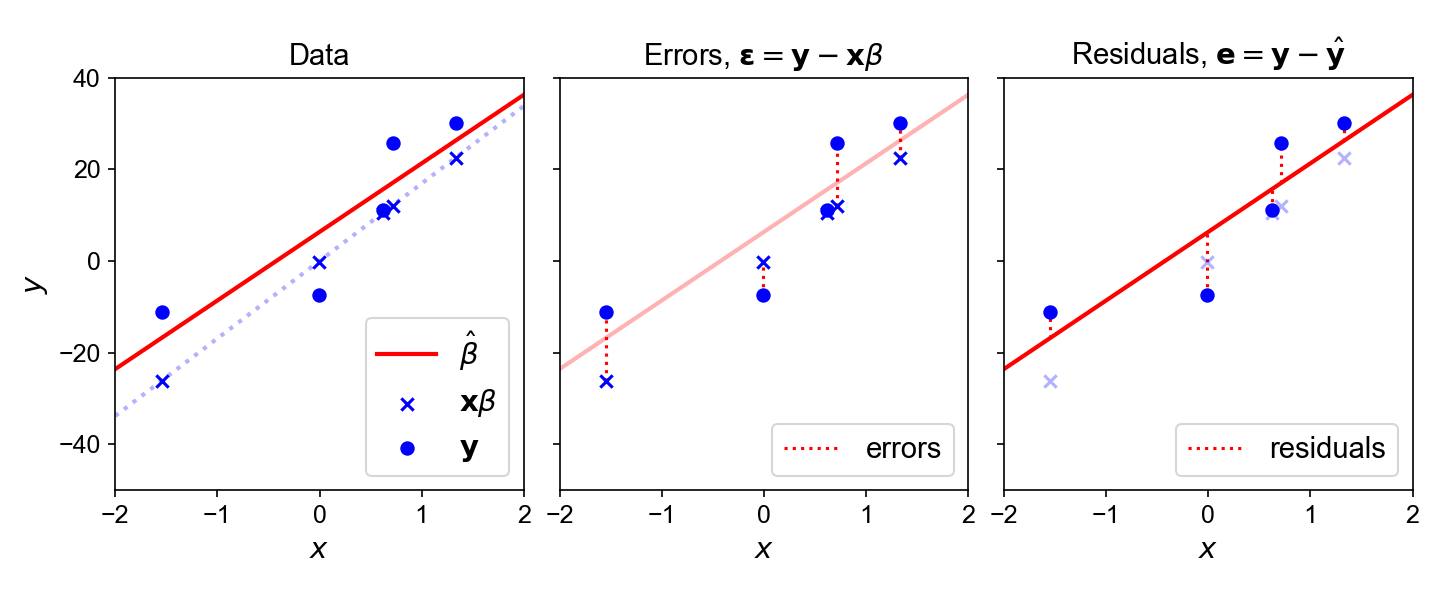
Thus, errors are related to the true data generating process $\mathbf{X}\mathbf{\beta }$, while residuals are related to the estimated model $\mathbf{X}\hat{\mathbf{\beta }}$ (Figure $1$). Clearly, if $\hat{\mathbf{y}}=\mathbf{y}$, then the residuals are zero.

Figure 1. (Left) Ground-truth (un-observed) univariate data $\mathbf{x}\beta$, noisy observations $\mathbf{y}=\mathbf{x}\beta +\mathbf{\epsilon }$, and estimated $\hat{\beta }$. (Middle) Errors $\mathbf{\epsilon }$ between ground-truth data $\mathbf{x}\beta$ and noisy observations $\mathbf{y}$. (Right) Residuals $\mathbf{e}$ between noisy observations $\mathbf{y}$ and model predictions $\hat{\mathbf{y}}=\mathbf{x}\hat{\beta }$.

Normal equation

Now that we understand the basic model, let’s discuss solving for $\mathbf{\beta }$. Since $\mathbf{X}$ is a tall and skinny matrix, solving for $\mathbf{\beta }$ amounts to solving a linear system of $N$ equations with $P$ unknowns. Such a system is overdetermined, and it is unlikely that such a system has an exact solution. Classical linear regression is sometimes called ordinary least squares (OLS) because the best-fit coefficients $[{\beta }_1,\dots ,{\beta }_P{]}^{\top }$ are defined as those that solve the following minimization problem:

$$\hat{\mathbf{\beta }}=\arg \underset{\mathbf{\beta }}{\min }\sum _{n=1}^N{\left(y_n-{\mathbf{x}}_n^{\top }\mathbf{\beta }\right)}^2.\text{\hspace{1em}(7)}$$

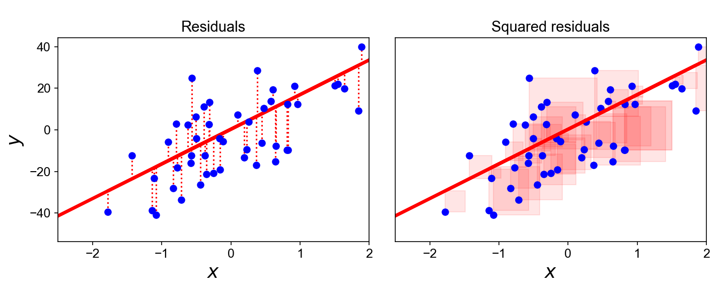
Thus, the OLS estimator $\hat{\mathbf{\beta }}$ minimizes the sum of squared residuals (Figure $2$). For a single data point, the squared error is zero if the prediction is exactly correct. Otherwise, the penalty increases quadratically, meaning classical linear regression heavily penalizes outliers. Other loss functions induce other linear models. See my previous post on interpreting these kinds of optimization problems.

Figure 2. Ordinary least squares linear regression on Scikit-learn's make_regression dataset. Data points are in blue. The predicted hyperplane is the red line. (Left) Red dashed vertical lines represent the residuals. (Right) Light red boxes represent the squared residuals.

In vector form, Equation $7$ is

$$\hat{\mathbf{\beta }}=\arg \underset{\mathbf{\beta }}{\min }\Vert \mathbf{y}-\mathbf{X}\mathbf{\beta }{\Vert }_2^2.\text{\hspace{1em}(8)}$$

Linear regression has an analytic or closed-form solution known as the normal equation,

$$\hat{\mathbf{\beta }}=({\mathbf{X}}^{\top }\mathbf{X}{)}^{-1}{\mathbf{X}}^{\top }\mathbf{y}.\text{\hspace{1em}(9)}$$

See A1 for a complete derivation of Equation $9$.

Hat matrix and residual maker

We’ll see in a moment where the name “normal equation” comes from. However, we must first understand some basic properties of OLS. Let’s define a matrix $\mathbf{H}$ as

$$\mathbf{H}\triangleq \mathbf{X}({\mathbf{X}}^{\top }\mathbf{X}{)}^{-1}{\mathbf{X}}^{\top }.\text{\hspace{1em}(10)}$$

We’ll call this the hat matrix, since it “puts a hat” on $\mathbf{y}$, i.e. since it regresses the response variables $\mathbf{y}$ onto the predicted variables $\hat{\mathbf{y}}$:

$$\begin{array}{rl}& \mathbf{H}\mathbf{y}\\ & =\mathbf{X}({\mathbf{X}}^{\top }\mathbf{X}{)}^{-1}{\mathbf{X}}^{\top }\mathbf{y}\\ & \stackrel{\star }{=}\mathbf{X}\hat{\mathbf{\beta }}\\ & =\hat{\mathbf{y}}\end{array}\text{\hspace{1em}(11)}$$

Step $\star$ is just the normal equation (Equation $8$). Note that $\mathbf{H}$ is an orthogonal projection. See A2 for a proof. Furthermore, let’s call

$$\mathbf{M}\triangleq \mathbf{I}-\mathbf{H}\text{\hspace{1em}(12)}$$

the residual maker since it constructs the residuals, i.e. since it makes the residuals from the response variables $\mathbf{y}$:

$$\begin{array}{rl}\mathbf{M}\mathbf{y}& =(\mathbf{I}-\mathbf{H})\mathbf{y}\\ & =\mathbf{y}-\mathbf{H}\mathbf{y}\\ & =\mathbf{y}-\hat{\mathbf{y}}\\ & =\mathbf{e}.\end{array}\text{\hspace{1em}(13)}$$

The residual maker is also an orthogonal projector. See A3 for a proof.

Finally, note that $\mathbf{H}$ and $\mathbf{M}$ are orthogonal to each other:

$$\begin{array}{rl}\mathbf{H}\mathbf{M}& =\mathbf{H}(\mathbf{I}-\mathbf{H})\\ & =\mathbf{H}-\mathbf{H}\\ & =0.\end{array}\text{\hspace{1em}(14)}$$

Geometric view of OLS

There is a nice geometric interpretation to all this. When we multiply the response variables $\mathbf{y}$ by $\mathbf{H}$, we are projecting $\mathbf{y}$ into a space spanned by the columns of $\mathbf{X}$. This makes sense since the model is constrained to live in the space of linear combinations of the columns of $\mathbf{X}$,

$$\mathbf{y}={\beta }_1\left[\begin{array}{c}{x}_{1,1}\\ x_{2,1}\\ ⋮\\ x_{N,1}\end{array}\right]+{\beta }_2\left[\begin{array}{c}{x}_{1,2}\\ x_{2,2}\\ ⋮\\ x_{N,2}\end{array}\right]+\cdots +{\beta }_P\left[\begin{array}{c}{x}_{1,P}\\ x_{2,P}\\ ⋮\\ x_{N,P}\end{array}\right]\text{\hspace{1em}(15)}$$

and an orthogonal projection is the closest to $\mathbf{y}$ in Euclidean distance that we can get while staying in this constrained space. (One can find many nice visualizations of this fact online.) I’m pretty sure this is why the normal equation is so-named, since “normal” is another word for “perpendicular” in geometry.

Thus, we can summarize the predictions made by OLS (Equation $4$) by saying that we project our response variables onto a linear hyperplane defined by $\hat{\mathbf{\beta }}$ using the orthogonal projection matrix $\mathbf{H}$.

OLS with an intercept

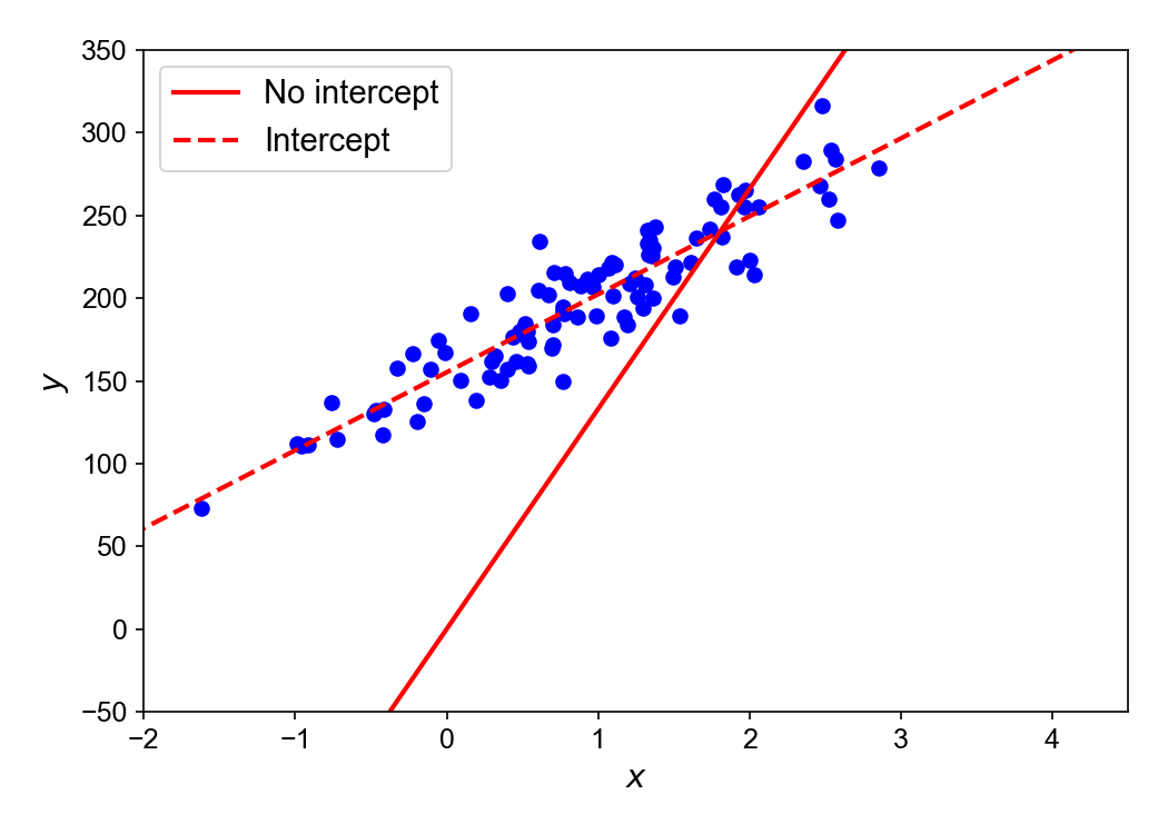
Notice that Equation $1$ does not include an intercept. In other words, our linear model is constrained such that the hyperplane $\hat{\mathbf{\beta }}$ goes through the origin. However, we often want to model a shift in the response variable, since this can dramatically improve the goodness-of-fit in the model (Figure $3$). Thus, we want OLS with an intercept.

Figure 3. OLS without (red solid line) and with (red dashed line) an intercept. The model's goodness-of-fit changes dramatically depending on this modeling assumption.

In this section, I’ll discuss both partitioned regression or OLS when the predictors and corresponding coefficients can be logically separated into groups via block matrices and then use that result for the specific case when one of the block matrices in the design matrix $\mathbf{X}$ is a constant, i.e. a constant term for an intercept.

Partitioned regression

Let’s rewrite Equation $3$ by splitting $\mathbf{X}$ and $\mathbf{\beta }$ into block matrices. Let $\mathbf{X}=[{\mathbf{X}}_1,{\mathbf{X}}_2]$ (we’re stacking the columns horizontally) and $\mathbf{\beta }=[{\mathbf{\beta }}_1,{\mathbf{\beta }}_2{]}^{\top }$ (we’re stacking the rows vertically). Then partitioned regression is,

$$\mathbf{y}=\left[\begin{array}{cc}{\mathbf{X}}_1& {\mathbf{X}}_2\end{array}\right]\left[\begin{array}{c}{\mathbf{\beta }}_1\\ {\mathbf{\beta }}_2\end{array}\right]+\mathbf{\epsilon }.\text{\hspace{1em}(16)}$$

The normal equation (Equation $9$) can then be written as

$$\left[\begin{array}{c}{\mathbf{X}}_1^{\top }\\ {\mathbf{X}}_2^{\top }\end{array}\right]\left[\begin{array}{cc}{\mathbf{X}}_1& {\mathbf{X}}_2\end{array}\right]\left[\begin{array}{c}{\hat{\mathbf{\beta }}}_1\\ {\hat{\mathbf{\beta }}}_2\end{array}\right]=\left[\begin{array}{c}{\mathbf{X}}_1^{\top }\\ {\mathbf{X}}_2^{\top }\end{array}\right]\mathbf{y},\text{\hspace{1em}(17)}$$

which in turn can be written as two separate equations:

$$\begin{array}{rl}{\mathbf{X}}_1^{\top }{\mathbf{X}}_1{\hat{\mathbf{\beta }}}_1+{\mathbf{X}}_1^{\top }{\mathbf{X}}_2{\hat{\mathbf{\beta }}}_2& ={\mathbf{X}}_1^{\top }\mathbf{y},\\ {\mathbf{X}}_2^{\top }{\mathbf{X}}_1{\hat{\mathbf{\beta }}}_1+{\mathbf{X}}_2^{\top }{\mathbf{X}}_2{\hat{\mathbf{\beta }}}_2& ={\mathbf{X}}_2^{\top }\mathbf{y}.\end{array}\text{\hspace{1em}(18)}$$

We can then solve for ${\hat{\mathbf{\beta }}}_1$ and ${\hat{\mathbf{\beta }}}_2$, since we have two equations and two unknowns. Let’s first solve for ${\hat{\mathbf{\beta }}}_1$. We have

$$\begin{array}{rl}{\mathbf{X}}_1^{\top }{\mathbf{X}}_1{\hat{\mathbf{\beta }}}_1& ={\mathbf{X}}_1^{\top }\mathbf{y}-{\mathbf{X}}_1^{\top }{\mathbf{X}}_2{\hat{\mathbf{\beta }}}_2\\ {\hat{\mathbf{\beta }}}_1& =({\mathbf{X}}_1^{\top }{\mathbf{X}}_1{)}^{-1}{\mathbf{X}}_1^{\top }(\mathbf{y}-{\mathbf{X}}_2{\hat{\mathbf{\beta }}}_2).\end{array}\text{\hspace{1em}(19)}$$

We can then isolate ${\hat{\mathbf{\beta }}}_2$ by substituting ${\hat{\mathbf{\beta }}}_1$ into the second line of Equation $18$:

$$\begin{array}{rl}{\mathbf{X}}_2^{\top }\mathbf{y}& ={\mathbf{X}}_2^{\top }{\mathbf{X}}_1{\hat{\mathbf{\beta }}}_1+{\mathbf{X}}_2^{\top }{\mathbf{X}}_2{\hat{\mathbf{\beta }}}_2\\ {\mathbf{X}}_2^{\top }\mathbf{y}& ={\mathbf{X}}_2^{\top }{\mathbf{X}}_1({\mathbf{X}}_1^{\top }{\mathbf{X}}_1{)}^{-1}{\mathbf{X}}_1^{\top }(\mathbf{y}-{\mathbf{X}}_2{\hat{\mathbf{\beta }}}_2)+{\mathbf{X}}_2^{\top }{\mathbf{X}}_2{\hat{\mathbf{\beta }}}_2\\ {\mathbf{X}}_2^{\top }\mathbf{y}& ={\mathbf{X}}_2^{\top }{\mathbf{X}}_1({\mathbf{X}}_1^{\top }{\mathbf{X}}_1{)}^{-1}{\mathbf{X}}_1^{\top }\mathbf{y}+\left\{{\mathbf{X}}_2^{\top }{\mathbf{X}}_2-{\mathbf{X}}_2^{\top }{\mathbf{X}}_1({\mathbf{X}}_1^{\top }{\mathbf{X}}_1{)}^{-1}{\mathbf{X}}_1^{\top }{\mathbf{X}}_2\right\}{\hat{\mathbf{\beta }}}_2.\end{array}\text{\hspace{1em}(20)}$$

If we define ${\mathbf{H}}_1$ and ${\mathbf{M}}_1$—hat and residual matrices for ${\mathbf{X}}_1$—as

$$\begin{array}{rl}{\mathbf{H}}_1& \triangleq {\mathbf{X}}_1({\mathbf{X}}_1^{\top }{\mathbf{X}}_1{)}^{-1}{\mathbf{X}}_1^{\top },\\ {\mathbf{M}}_1& \triangleq \mathbf{I}-{\mathbf{H}}_1,\end{array}\text{\hspace{1em}(21)}$$

then Equation $20$ can be rewritten as:

$$\begin{array}{rl}\left\{{\mathbf{X}}_2^{\top }{\mathbf{X}}_2-{\mathbf{X}}_2^{\top }{\mathbf{X}}_1({\mathbf{X}}_1^{\top }{\mathbf{X}}_1{)}^{-1}{\mathbf{X}}_1^{\top }{\mathbf{X}}_2\right\}{\hat{\mathbf{\beta }}}_2& ={\mathbf{X}}_2^{\top }\mathbf{y}-{\mathbf{X}}_2^{\top }{\mathbf{X}}_1({\mathbf{X}}_1^{\top }{\mathbf{X}}_1{)}^{-1}{\mathbf{X}}_1^{\top }\mathbf{y},\\ & \Downarrow \\ \left\{{\mathbf{X}}_2^{\top }\left(\mathbf{I}-{\mathbf{H}}_1\right){\mathbf{X}}_2\right\}{\hat{\mathbf{\beta }}}_2& ={\mathbf{X}}_2^{\top }\left(\mathbf{I}-{\mathbf{H}}_1\right)\mathbf{y}.\end{array}\text{\hspace{1em}(22)}$$

And we have solved for ${\hat{\mathbf{\beta }}}_2$ in terms of the residual maker for ${\mathbf{X}}_1$, denoted ${\mathbf{M}}_1$:

$${\hat{\mathbf{\beta }}}_2={\left({\mathbf{X}}_2^{\top }{\mathbf{M}}_1{\mathbf{X}}_2\right)}^{-1}{\mathbf{X}}_2^{\top }{\mathbf{M}}_1\mathbf{y}.\text{\hspace{1em}(23)}$$

As we’ll see in the next section, solving for ${\hat{\mathbf{\beta }}}_2$ in terms of ${\mathbf{M}}_1$ will be make it easier to understand and compute the optimal parameters of OLS with an intercept.

The results in Equations $19$ and $23$ are part of the Frisch–Waugh–Lovell (FWL) theorem. The basic idea of the FWL theorem is that we can obtain ${\hat{\mathbf{\beta }}}_2$ by regressing ${\mathbf{M}}_1\mathbf{y}$ onto ${\mathbf{M}}_1{\mathbf{X}}_2$, where these variables are just the residuals associated with ${\mathbf{X}}_1$. See (Greene, 2003) for further discussion.

Partitioned regression with a constant predictor

OLS with an intercept is just a special case of partitioned regression. Suppose that we add an intercept to our OLS model. This means we want to estimate a new parameter ${\beta }_0$ such that

$$y_n={\beta }_0+{\mathbf{x}}_n^{\top }\mathbf{\beta }+{\epsilon }_n.\text{\hspace{1em}(24)}$$

Notice that if we simply add a constant to our predictor ${\mathbf{x}}_n$, we can “push” ${\beta }_0$ into the dot product. In matrix notation, we have

$$\mathbf{y}=\left[\begin{array}{cccc}1& x_{11}& \dots & x_{1P}\\ 1& x_{21}& \dots & x_{2P}\\ ⋮& ⋮& \ddots & ⋮\\ 1& x_{N1}& \dots & x_{NP}\end{array}\right]\left[\begin{array}{c}{\beta }_0\\ {\beta }_1\\ ⋮\\ {\beta }_P\end{array}\right]+\mathbf{\epsilon },\text{\hspace{1em}(25)}$$

which is the same equation as Equation $3$ but with a column of ones prepended to $\mathbf{X}$. This means we can write our model as

$$\mathbf{y}=1{\beta }_1+{\mathbf{X}}_2{\mathbf{\beta }}_2+\mathbf{\epsilon }.\text{\hspace{1em}(26)}$$

We can use the results of the previous subsection to straightforwardly solve for the scalar ${\beta }_1$ and the $P$-vector ${\mathbf{\beta }}_2$. First, note that the hat matrix ${\mathbf{H}}_1$ is just an $N\times N$ matrix filled with the value $1/N$:

$$\begin{array}{rl}{\mathbf{H}}_1& =1(1^{\top }1)1^{\top }\\ & =\frac{1}{N}11^{\top }\\ & =\left[\begin{array}{ccc}1/N& \dots & 1/N\\ ⋮& \ddots & ⋮\\ 1/N& \dots & 1/N\end{array}\right]\end{array}.\text{\hspace{1em}(27)}$$

With this in mind, let’s compute ${\hat{\mathbf{\beta }}}_2$ using Equation $23$. We know that ${\mathbf{M}}_1\mathbf{y}=\hat{\mathbf{y}}$. Furthermore, we can simplify ${\mathbf{X}}_2^{\top }{\mathbf{M}}_1{\mathbf{X}}_2$ as

$$\begin{array}{rl}{\mathbf{X}}_2^{\top }{\mathbf{M}}_1{\mathbf{X}}_2& ={\mathbf{X}}_2^{\top }(\mathbf{I}-{\mathbf{H}}_1){\mathbf{X}}_2\\ & ={\mathbf{X}}_2^{\top }({\mathbf{X}}_2-{\mathbf{H}}_1{\mathbf{X}}_2)\\ & ={\mathbf{X}}_2^{\top }({\mathbf{X}}_2-{\bar{\mathbf{X}}}_2),\end{array}\text{\hspace{1em}(28)}$$

where ${\bar{\mathbf{X}}}_2$ is a matrix where each column is an $N$-vector with the mean of that respective column in ${\mathbf{X}}_2$ repeated $N$ times since

$${\bar{\mathbf{X}}}_2\triangleq \left[\begin{array}{ccc}1/N& \dots & 1/N\\ ⋮& \ddots & ⋮\\ 1/N& \dots & 1/N\end{array}\right]\left[\begin{array}{ccc}{x}_{11}& \dots & x_{1P}\\ ⋮& \ddots & ⋮\\ x_{N1}& \dots & x_{NP}\end{array}\right]=\left[\begin{array}{ccc}{\bar{x}}_{:,1}& \dots & {\bar{x}}_{:,P}\\ ⋮& \ddots & ⋮\\ {\bar{x}}_{:,1}& \dots & {\bar{x}}_{:,P}\end{array}\right],\text{\hspace{1em}(29)}$$

where ${\bar{x}}_{:,p}$ is defined as

$${\bar{x}}_{:,p}=\frac{1}{N}\sum _{n=1}^N{x}_{n,p},\text{\hspace{1em}(30)}$$

or the mean of a column of $\mathbf{X}$. Thus, we are just mean centering ${\mathbf{X}}_2$ in the calculation ${\mathbf{X}}_2-{\bar{\mathbf{X}}}_2$. This gives us

$$\begin{array}{rl}{\hat{\mathbf{\beta }}}_2& ={\left\{{\mathbf{X}}_2^{\top }({\mathbf{X}}_2-{\bar{\mathbf{X}}}_2)\right\}}^{-1}{\mathbf{X}}_2^{\top }(\mathbf{y}-\hat{\mathbf{y}}).\end{array}\text{\hspace{1em}(31)}$$

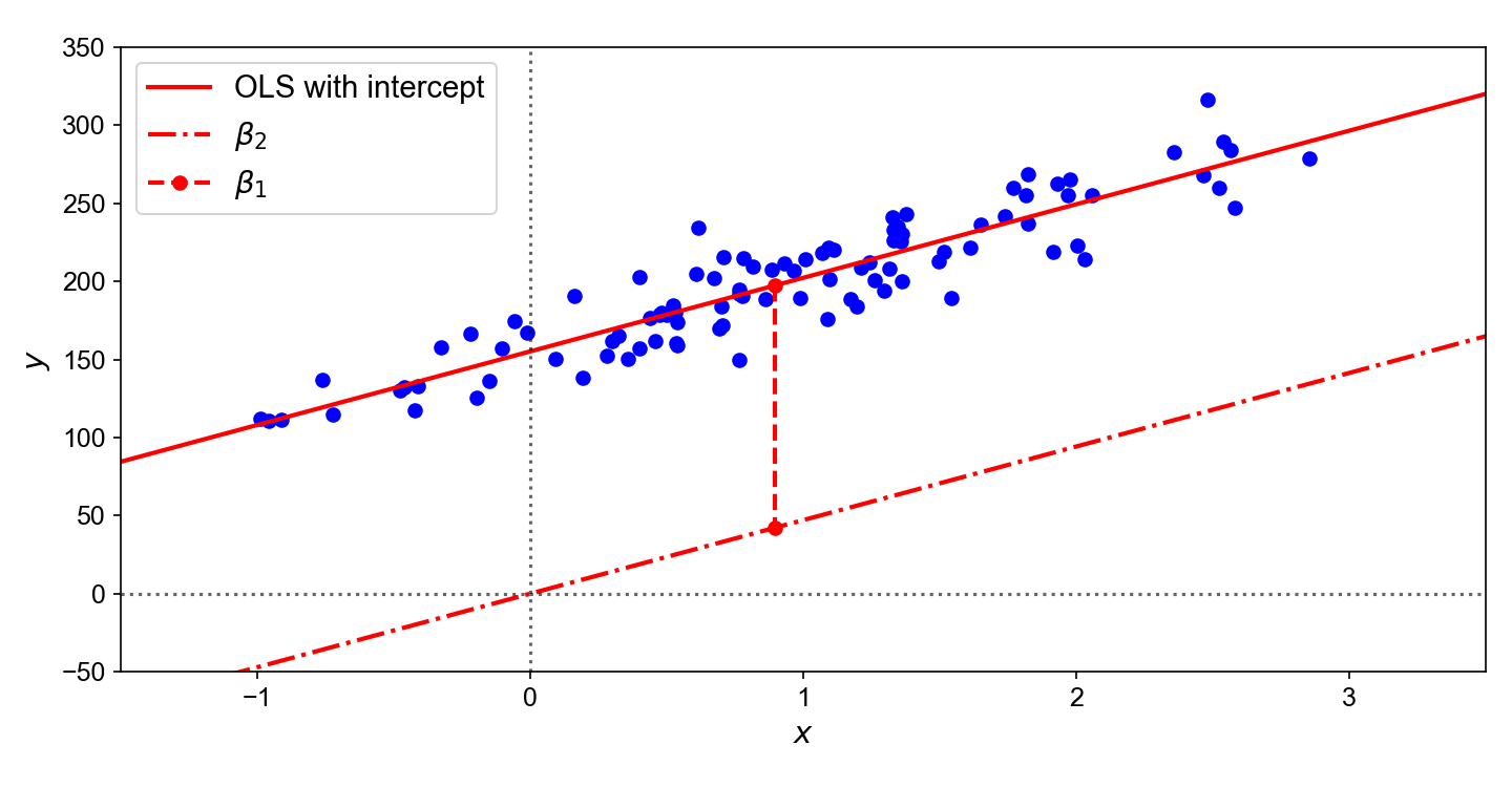
In other words, when OLS has an intercept, the optimal coefficients $\widehat{{\mathbf{\beta }}_2}$—which are the parameters associated with the predictors in our design matrix—are just the result of the normal equation after mean-centering our targets and predictors. Intuitively, this means that the hyperplane defined by just $\widehat{{\mathbf{\beta }}_2}$ goes through the origin (Figure $4$).

Figure 4. OLS with an intercept (solid line) can be decomposed into OLS without an intercept (dashed-and-dotted line) and a bias term (dashed line). Without an intercept, OLS goes through the origin. With an intercept, the hyperplane is shifted by the distance between the original hyperplane and the mean of the data.

Finally, we can solve for the scalar ${\hat{\beta }}_1$—which is really the intercept parameter ${\beta }_0$ in Equation $24$—as

$$\begin{array}{rl}{\hat{\beta }}_1& =(1^{\top }1{)}^{-1}{1}^{\top }(\mathbf{y}-{\mathbf{X}}_2{\hat{\mathbf{\beta }}}_2)\\ & =\frac{1}{N}{1}^{\top }(\mathbf{y}-{\mathbf{X}}_2{\hat{\mathbf{\beta }}}_2)\\ & =\bar{y}-{\bar{\mathbf{x}}}_2{\hat{\mathbf{\beta }}}_2,\end{array}\text{\hspace{1em}(32)}$$

where ${\bar{\mathbf{x}}}_2$ is a row of ${\bar{\mathbf{X}}}_2$, i.e. a vector of means for each predictor. The interpretation of this bias parameter (Equation $32$) becomes more clear if we diagram these quantities (Figure $4$). As we can see, OLS with an intercept can be decomposed into OLS without an intercept, where the hyperplane defined by ${\hat{\mathbf{\beta }}}_2$ passes through the origin, and the bias parameter ${\beta }_1$ (again elsewhere denoted ${\beta }_0$), which shifts the hyperplane from the origin to the mean of the response variables.

A probabilistic perspective

OLS can be viewed from a probabilistic perspective. Recall the linear model

$$y_n={\mathbf{x}}_n^{\top }\mathbf{\beta }+{\epsilon }_n.\text{\hspace{1em}(33)}$$

If we assume our error ${\epsilon }_n$ is additive Gaussian noise, ${\epsilon }_n\sim \mathcal{N}(0,{\sigma }^2)$, then this induces a conditionally Gaussian assumption on our response variables,

$$p(y_n\mid {\mathbf{x}}_n,\mathbf{\beta },{\sigma }^2)=\mathcal{N}(y_n\mid {\mathbf{x}}_n^{\top }\mathbf{\beta },{\sigma }^2).\text{\hspace{1em}(34)}$$

If our data is i.i.d., we can write

$$p(\mathbf{y}\mid \mathbf{x},\mathbf{\beta },{\sigma }^2)=\prod _{n=1}^N\mathcal{N}(y_n\mid {\mathbf{x}}_n^{\top }\mathbf{\beta },{\sigma }^2).\text{\hspace{1em}(35)}$$

In this statistical framework, maximum likelihood (ML) estimation gives us the same optimal parameters as the normal equation. To compute the ML estimate, we first take derivative with respect to the parameter of the log likelihood function and then solve for $\mathbf{\beta }$. We can represent the log likelihood compactly using a multivariate normal distribution,

$$\log p(\mathbf{y}\mid \mathbf{x},\mathbf{\beta },{\sigma }^2)=-\frac{N}{2}\log (2\pi {\sigma }^2)-\frac{1}{2{\sigma }^2}(\mathbf{y}-\mathbf{X}\mathbf{\beta }{)}^{\top }(\mathbf{y}-\mathbf{X}\mathbf{\beta })\text{\hspace{1em}(36)}$$

See A4 for a complete derivation of Equation $36$. If we take the derivative of this log likelihood function with respect to the parameters, the first term is zero and the constant $1/2{\sigma }^2$ does not effect our optimization. Thus, we are looking for

$${\hat{\mathbf{\beta }}}_{\text{MLE}}=\arg \underset{\mathbf{\beta }}{\max }\{-(\mathbf{y}-\mathbf{X}\mathbf{\beta }{)}^{\top }(\mathbf{y}-\mathbf{X}\mathbf{\beta })\}.\text{\hspace{1em}(37)}$$

Of course, maximizing the negation of a function is the same as minimizing the function directly. Thus, this is the same optimization problem as Equations $7$ and $8$.

Furthermore, let ${\mathbf{\beta }}_0$ and ${\sigma }_0^2$ be the true generative parameters. Then

$$\begin{array}{rl}\mathbb{E}[\mathbf{y}\mid \mathbf{X}]& =\mathbf{X}{\mathbf{\beta }}_0\\ \mathbb{V}[\mathbf{y}\mid \mathbf{X}]& ={\sigma }_0^2\mathbf{I}.\end{array}\text{\hspace{1em}(38)}$$

See A5 for a derivation of Equation $38$. Since we know that the conditional expectation is the minimizer of the mean squared loss—see my previous post if needed—, we know that $\mathbf{X}{\mathbf{\beta }}_0$ would be the best we can do given our model. An interpretation of the conditional variance in this context is that it is the smallest expected squared prediction error.

Conclusion

Classical linear regression or ordinary least squares is a linear model in which the estimated parameters minimize the sum of squared residuals. Geometrically, we can interpret OLS as orthogonally projecting our response variables onto a hyperplane defined by these linear coefficients. OLS typically includes an intercept, which shifts the hyperplane so that it goes through the targets’ mean, rather than through the origin. In a probabilistic view of OLS, the maximum likelihood estimator is equivalent to the solution to the normal equation.

Acknowledgements

I thank Andrei Margeloiu for correcting an error in an earlier version of this post. When $\hat{\mathbf{y}}=\mathbf{y}$, the residuals are zero, but the true errors are still unknown.

Appendix

A1. Normal equation

We want to find the parameters or coefficients $\mathbf{\beta }$ that minimize the sum of squared residuals,

$$\hat{\mathbf{\beta }}=\arg \underset{\mathbf{\beta }}{\min }\Vert \mathbf{y}-\mathbf{X}\mathbf{\beta }{\Vert }_2^2.\text{\hspace{1em}(A1.1)}$$

Note that we can write

$$\Vert \mathbf{y}-\mathbf{X}\mathbf{\beta }{\Vert }_2^2=(\mathbf{y}-\mathbf{X}\mathbf{\beta }{)}^{\top }(\mathbf{y}-\mathbf{X}\mathbf{\beta }).\text{\hspace{1em}(A1.2)}$$

This can be easily seen by writing out the vectorization explicitly. Let $\mathbf{v}$ be a vector such that

$$\mathbf{v}=\left[\begin{array}{c}{y}_1-{\mathbf{x}}_1^{\top }\mathbf{\beta }\\ ⋮\\ y_N-{\mathbf{x}}_N^{\top }\mathbf{\beta }\end{array}\right]=\left[\begin{array}{c}{y}_1\\ ⋮\\ y_N\end{array}\right]-\left[\begin{array}{ccc}{x}_{11}& \dots & x_{1P}\\ ⋮& \ddots & ⋮\\ x_{N1}& \dots & x_{NP}\end{array}\right]\left[\begin{array}{c}{\beta }_1\\ \dots \\ {\beta }_P\end{array}\right].\text{\hspace{1em}(A1.3)}$$

The squared L2-norm $\Vert \mathbf{v}{\Vert }_2^2$ is the sums the squared components of $\mathbf{v}$. This is equivalent to taking the dot product ${\mathbf{v}}^{\top }\mathbf{v}$. Now define the function $J(\cdot )$ such that

$$J(\mathbf{\beta })=\Vert \mathbf{y}-\mathbf{X}\mathbf{\beta }{\Vert }_2^2.\text{\hspace{1em}(A1.4)}$$

To minimize $J(\cdot )$, we take its derivative with respect to $\mathbf{\beta }$, set it equal to zero, and solve for $\mathbf{\beta }$,

$$\begin{array}{rl}{\nabla }_{\mathbf{\beta }}J(\mathbf{\beta })& \stackrel{1}{=}{\nabla }_{\mathbf{\beta }}[(\mathbf{y}-\mathbf{X}\mathbf{\beta }{)}^{\top }(\mathbf{y}-\mathbf{X}\mathbf{\beta })]\\ & \stackrel{2}{=}{\nabla }_{\mathbf{\beta }}[({\mathbf{y}}^{\top }-{\mathbf{\beta }}^{\top }{\mathbf{X}}^{\top })(\mathbf{y}-\mathbf{X}\mathbf{\beta })]\\ & \stackrel{3}{=}{\nabla }_{\mathbf{\beta }}[{\mathbf{\beta }}^{\top }{\mathbf{X}}^{\top }\mathbf{X}\mathbf{\beta }-{\mathbf{y}}^{\top }\mathbf{X}\mathbf{\beta }+{\mathbf{y}}^{\top }\mathbf{y}-{\mathbf{\beta }}^{\top }{\mathbf{X}}^{\top }\mathbf{y}]\\ & \stackrel{4}{=}{\nabla }_{\mathbf{\beta }}\text{tr}({\mathbf{\beta }}^{\top }{\mathbf{X}}^{\top }\mathbf{X}\mathbf{\beta }-{\mathbf{y}}^{\top }\mathbf{X}\mathbf{\beta }+{\mathbf{y}}^{\top }\mathbf{y}-{\mathbf{\beta }}^{\top }{\mathbf{X}}^{\top }\mathbf{y})\\ & \stackrel{5}{=}{\nabla }_{\mathbf{\beta }}\text{tr}\left({\mathbf{\beta }}^{\top }{\mathbf{X}}^{\top }\mathbf{X}\mathbf{\beta }\right)-{\nabla }_{\mathbf{\beta }}\text{tr}\left({\mathbf{y}}^{\top }\mathbf{X}\mathbf{\beta }\right)+\cancel{{\nabla }_{\mathbf{\beta }}\text{tr}\left({\mathbf{y}}^{\top }\mathbf{y}\right)}-{\nabla }_{\mathbf{\beta }}\text{tr}\left({\mathbf{\beta }}^{\top }{\mathbf{X}}^{\top }\mathbf{y}\right)\\ & \stackrel{6}{=}{\nabla }_{\mathbf{\beta }}\text{tr}\left({\mathbf{\beta }}^{\top }{\mathbf{X}}^{\top }\mathbf{X}\mathbf{\beta }\right)-2{\nabla }_{\mathbf{\beta }}\text{tr}\left({\mathbf{\beta }}^{\top }{\mathbf{X}}^{\top }\mathbf{y}\right)\\ & \stackrel{7}{=}2{\mathbf{X}}^{\top }\mathbf{X}\mathbf{\beta }-2{\mathbf{X}}^{\top }\mathbf{y}\end{array}\text{\hspace{1em}(A1.5)}$$

In step $4$, we use the fact that the trace of a scalar is the scalar. In step $5$, we use the linearity of differentiation and the trace operator. In step $6$, we use the fact that $\text{tr}(\mathbf{A})=\text{tr}({\mathbf{A}}^{\top })$. In step $7$, we take the derivatives of the left and right terms using identities $108$ and $103$ from (Petersen et al., 2008), respectively.

If we set line $7$ equal to zero and divide both sides of the equation by two, we get the normal equation:

$${\mathbf{X}}^{\top }\mathbf{X}\mathbf{\beta }={\mathbf{X}}^{\top }\mathbf{y}.\text{\hspace{1em}(A1.6)}$$

A2. Hat matrix is an orthogonal projection

A square matrix is a projection if $\mathbf{A}={\mathbf{A}}^2$. Thus, the hat matrix $\mathbf{H}$ is a projection since

$$\begin{array}{rl}{\mathbf{H}}^2& =\mathbf{H}\mathbf{H}\\ & =\left(\mathbf{X}({\mathbf{X}}^{\top }\mathbf{X}{)}^{-1}{\mathbf{X}}^{\top }\right)\left(\mathbf{X}({\mathbf{X}}^{\top }\mathbf{X}{)}^{-1}{\mathbf{X}}^{\top }\right)\\ & =\mathbf{X}({\mathbf{X}}^{\top }\mathbf{X}{)}^{-1}{\mathbf{X}}^{\top }\\ & =\mathbf{H}.\end{array}\text{\hspace{1em}(A2.1)}$$

A real-valued projection is orthogonal if $\mathbf{A}={\mathbf{A}}^{\top }$. Thus, the hat matrix $\mathbf{H}$ is an orthogonal projection since

$$\begin{array}{rl}{\mathbf{H}}^{\top }& =(\mathbf{X}({\mathbf{X}}^{\top }\mathbf{X}{)}^{-1}{\mathbf{X}}^{\top }{)}^{\top }\\ & =({\mathbf{X}}^{\top }{)}^{\top }[({\mathbf{X}}^{\top }\mathbf{X}{)}^{-1}{]}^{\top }{\mathbf{X}}^{\top }\\ & =\mathbf{H}.\end{array}\text{\hspace{1em}(A2.2)}$$

A3. Residual maker is an orthogonal projector

A square matrix $\mathbf{A}$ is a projection if $\mathbf{A}={\mathbf{A}}^2$. For the residual maker $\mathbf{M}$, we have:

$$\begin{array}{rl}{\mathbf{M}}^2& =(\mathbf{I}-\mathbf{H})(\mathbf{I}-\mathbf{H})\\ & =\mathbf{I}-\mathbf{H}-\mathbf{H}+{\mathbf{H}}^2\\ & \stackrel{\star }{=}\mathbf{I}-\mathbf{H}\\ & =\mathbf{M}.\end{array}\text{\hspace{1em}(A3.1)}$$

Step $\star$ holds because we know that the hat matrix $\mathbf{H}$ is an orthogonal projector. A real-valued projection $\mathbf{A}$ is orthogonal if $\mathbf{A}={\mathbf{A}}^{\top }$. For the residual maker $\mathbf{M}$, we have:

$$\begin{array}{rl}{\mathbf{M}}^{\top }& =(\mathbf{I}-\mathbf{H}{)}^{\top }\\ & ={\mathbf{I}}^{\top }-{\mathbf{H}}^{\top }\\ & \stackrel{†}{=}\mathbf{I}-\mathbf{H}.\end{array}\text{\hspace{1em}(A3.2)}$$

Again, step $†$ holds because $\mathbf{H}$ is an orthogonal projector. Therefore, $\mathbf{M}$ is an orthogonal projector.

A4. Multivariate normal representation of the log likelihood

The probability density function for a $D$-dimensional multivariate normal distribution is

$$p(\mathbf{z}\mid \mathbf{\mu },\mathbf{\Sigma })=\frac{1}{\sqrt{(2\pi {)}^D\det (\mathbf{\Sigma })}}\exp \{-\frac{1}{2}(\mathbf{z}-\mathbf{\mu }{)}^{\top }{\mathbf{\Sigma }}^{-1}(\mathbf{z}-\mathbf{\mu })\}.\text{\hspace{1em}(A4.1)}$$

The mean parameter $\mathbf{\mu }$ is a $D$-vector, and the covariance matrix $\mathbf{\Sigma }$ is a $D\times D$ positive definite matrix. In the probabilistic view of classical linear regression, the data are i.i.d. Therefore, we can represent the likelihood function as

$$p(\mathbf{y}\mid \mathbf{X},\mathbf{\beta },{\sigma }^2)=\frac{1}{\sqrt{(2\pi {\sigma }^2{)}^N}}\exp \{-\frac{1}{2{\sigma }^2}(\mathbf{y}-\mathbf{X}\mathbf{\beta }{)}^{\top }(\mathbf{y}-\mathbf{X}\mathbf{\beta })\}.\text{\hspace{1em}(A4.2)}$$

The above formulation leverages two properties from linear alegbra. First, if the dimensions of the covariance matrix are independent (in our case, each dimension is a sample), then $\mathbf{\Sigma }$ is diagonal, and its matrix inverse is just a diagonal matrix with each value replaced by its reciprocal. Second, the determinant of a diagonal matrix is just the product of the diagonal elements.

The log likelihood is then

$$\log p(\mathbf{y}\mid \mathbf{X},\mathbf{\beta },{\sigma }^2)=-\frac{N}{2}\log (2\pi {\sigma }^2)-\frac{1}{2{\sigma }^2}(\mathbf{y}-\mathbf{X}\mathbf{\beta }{)}^{\top }(\mathbf{y}-\mathbf{X}\mathbf{\beta })\text{\hspace{1em}(A4.3)}$$

as desired.

A5. Conditional expectation and variance

$$\begin{array}{rl}\mathbb{E}[\mathbf{y}\mid \mathbf{X}]& =\mathbb{E}[\mathbf{X}{\mathbf{\beta }}_0+\mathbf{\epsilon }\mid \mathbf{X}]\\ & =\mathbb{E}[\mathbf{X}{\mathbf{\beta }}_0\mid \mathbf{X}]+\mathbb{E}[\mathbf{\epsilon }\mid \mathbf{X}]\\ & =\mathbf{X}{\mathbf{\beta }}_0+\mathbb{E}[\mathbf{\epsilon }]\\ & =\mathbf{X}{\mathbf{\beta }}_0,\\ & \\ \mathbb{V}[\mathbf{y}\mid \mathbf{X}]& =\mathbb{V}[\mathbf{X}{\mathbf{\beta }}_0+\mathbf{\epsilon }\mid \mathbf{X}]\\ & =\mathbb{V}[\mathbf{X}{\mathbf{\beta }}_0\mid \mathbf{X}]+\mathbb{V}[\mathbf{\epsilon }\mid \mathbf{X}]\\ & =\mathbb{V}[\mathbf{X}\mid \mathbf{X}]+\mathbb{V}[\mathbf{\epsilon }]\\ & ={\sigma }_0^2\mathbf{I}.\end{array}\text{\hspace{1em}(A5.1)}$$