Implicit Lifting and the Kernel Trick

Implicit lifting

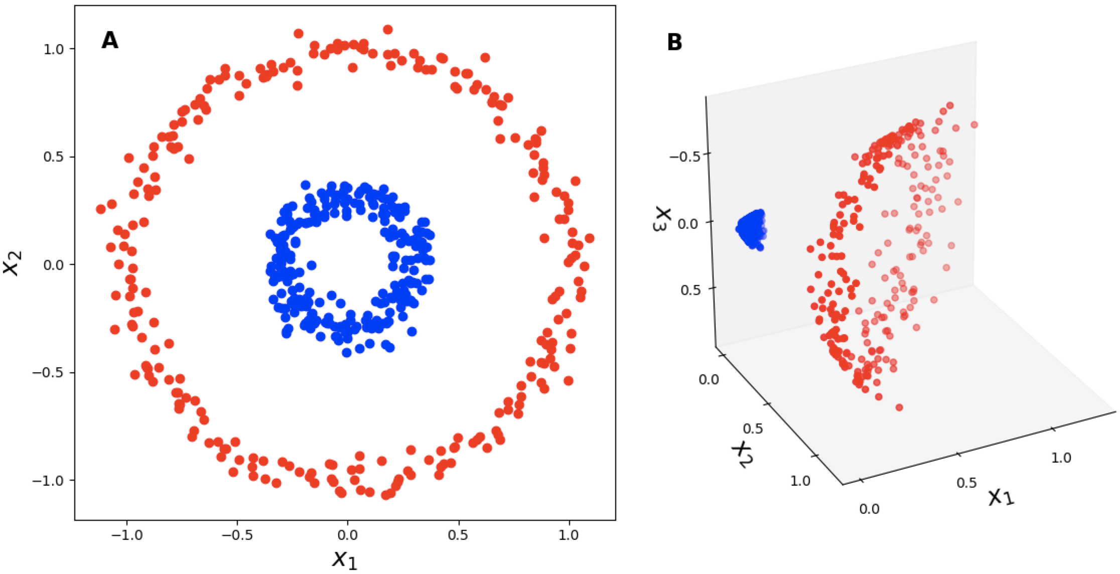
Imagine we have some data for a classification problem that is not linearly separable. A classic example is Figure $1$a. We would like to use a linear classifier. How might we do this? One idea is to augment our data’s features so that we can “lift” it into a higher dimensional space in which our data are linearly separable (Figure $1$b).

Figure 1: The "lifting trick". (a) A binary classification problem that is not linearly separable in $\mathbb{R}^2$. (b) A lifting of the data into $\mathbb{R}^3$ using a polynomial kernel, $\varphi([x_1 \;\; x_2]) = [x_1^2 \;\; x_2^2 \;\; \sqrt{2} x_1 x_2]$.

Let’s formalize this approach. Let our data be $\{(\mathbf{x}_1, y_1), \dots, (\mathbf{x}_N, y_N)\}$ where $\mathbf{x}_n \in \mathbb{R}^D$ in general. Now consider $D = 2$ and a single data point

$\mathbf{x} = \begin{bmatrix} x_1 \\ x_2 \end{bmatrix}.$

We might transform each data point with a function (the polynomial kernel for the curious),

$\varphi(\mathbf{x}) = \begin{bmatrix} x_1^2 \\ x_2^2 \\ \sqrt{2} x_1 x_2 \end{bmatrix}.$

Since our new data, $\varphi(\mathbf{x})$, is in $\mathbb{R}^3$, we might be able to find a hyperplane $\boldsymbol{\beta}$ in 3D to separate our observations,

$\boldsymbol{\beta}^{\top} \varphi(\mathbf{x}) = \beta_0 + \beta_1 x_1^2 + \beta_2 x_2^2 + \beta_3 \sqrt{2} x_1 x_2 = 0.$

This idea, while cool, is not the kernel trick, but it deserves a name. Rather than calling it the pre-(kernel trick) trick, let’s just call it the lifting trick. Caveat: I am not aware of a name for this trick, but I find naming things useful. If you loudly call this “the lifting trick” at a machine-learning party, you might get confused looks.

In order to find this hyperplane, we need to run a classification algorithm on our data after it has been lifted into three-dimensional space. At this point, we could be done. We take $\mathbb{R}^D$, perform our lifting trick into $\mathbb{R}^J$ where $D < J$, and then use a method like logistic regression to try to linearly classify it. However, this might be expensive for a “fancy” enough $\varphi(\cdot)$. For $N$ data points lifted into $J$ dimensions, we need $NJ$ operations just to preprocess the data. But we can avoid computing $\varphi(\cdot)$ entirely while still doing linear classification in this lifted space if we’re clever. This second trick is the kernel trick.

The kernel trick

Consider the loss function for a support vector machine (SVM):

$L(\mathbf{w}, \boldsymbol{\alpha}) = \sum_n \alpha_n - \frac{1}{2} \sum_n^N \sum_m^N \alpha_n \alpha_m y_n y_m (\mathbf{x}_n^{\top} \mathbf{x}_m)$

$\mathbf{w}$ is a normed vector representing the linear decision boundary and $\boldsymbol{\alpha}$ is a vector of Lagrange multipliers. If this is new or confusing, please see these excellent lecture notes from Rob Schapire’s Princeton course on theoretical machine learning. Otherwise, you can elide the details if you like; the upshot is that SVMs require computing a dot product and that, as formulated, the SVM is linear. (Note that $\mathbf{w}$ is implicit in the equation above; see those lecture notes as needed.)

Now what if we had the data problem in Figure $1$a? Could we use the lifting trick to make our SVM nonlinear? Sure. For the previously specified $\varphi(\cdot)$, we have

$\begin{aligned} \varphi(\mathbf{x}_n)^{\top} \varphi(\mathbf{x}_m) &= \begin{bmatrix} x_{n,1}^2 & x_{n,2}^2 & \sqrt{2} x_{n,1} x_{n,2} \end{bmatrix} \cdot \begin{bmatrix} x_{m,1}^2 \\ x_{m,2}^2 \\ \sqrt{2} x_{m,1} x_{m,2} \end{bmatrix} \\ &= x_{n,1}^2 x_{m,1}^2 + x_{n,2}^2 x_{m,2}^2 + 2 x_{n,1} x_{n,2} x_{m,1} x_{m,2}. \end{aligned}$

We would then need to compute this for all our $N$ data points. As we discussed, the problem with this approach is scalability. However, consider the following derivation,

$\begin{aligned} (\mathbf{x}_n^{\top} \mathbf{x}_m)^2 &= \Big( \begin{bmatrix} x_{n,1} & x_{n,2} \end{bmatrix} \cdot \begin{bmatrix} x_{m,1} \\ x_{m,2} \end{bmatrix} \Big)^2 \\ &= (x_{n,1} x_{m,1} + x_{n,2} x_{m,2})^2 \\ &= (x_{n,1} x_{m,1})^2 + (x_{n,2} x_{m,2})^2 + 2(x_{n,1} x_{m,1})(x_{n,2} x_{m,2}) \\ &= \varphi(\mathbf{x}_n)^{\top} \varphi(\mathbf{x}_m). \end{aligned}$

What just happened? Rather than lifting our data into $\mathbb{R}^3$ and computing an inner product, we just computed an inner product in $\mathbb{R}^2$ and then squared the sum. While both derivations have a similar number of mathematical symbols, the actual number of operations is much smaller for the second approach. This is because a inner product in $\mathbb{R}^2$ is two multiplications and a sum. The square is just the square of a scalar, so 4 operations. The first approach squared three components of two vectors (6 operations), then performed an inner product (3 multiplications, 1 sum) for 9 operations.

This is the kernel trick: we can avoid expensive operations in high dimensions by finding an appropriate kernel function $k(\mathbf{x}_n,\mathbf{x}_m)$ that is equivalent to the inner product in higher dimensional space. In our example above, $k(\mathbf{x}_n, \mathbf{x}_m) = (\mathbf{x}_n^{\top} \mathbf{x}_m)^2$. In other words, the kernel trick performs the lifting trick for cheap.

Mercer’s theorem

The mathematical basis for the kernel trick was discovered by James Mercer. Mercer proved that any positive definition function $k(\mathbf{x}_n, \mathbf{x}_m)$ with $\mathbf{x}_n, \mathbf{x}_m \in \mathbb{R}^D$ defines an inner product of another vector space $\mathcal{V}$. Thus, if you have a function $\varphi(\cdot)$ such that $\langle \varphi(\mathbf{x}_n), \varphi(\mathbf{x}_m) \rangle_{\mathcal{V}}$ is a valid inner product in $\mathcal{V}$, you know a kernel function exists that can perform the lifting trick for cheap. Alternatively, if you have a positive definite kernel, you can deconstruct its implicit basis function $\varphi(\cdot)$.

This idea is formalized in Mercer’s Theorem (taken from Michael Jordan’s lecture notes){:target=”_blank”}:

Mercer’s Theorem: A symmetric function $k(\mathbf{x}, \mathbf{y})$ can be expressed as an inner product

$> k(\mathbf{x}, \mathbf{y}) = \langle \varphi(\mathbf{x}), \varphi(\mathbf{y}) \rangle >$

for some $\varphi(\cdot)$ if and only if $k(\mathbf{x}, \mathbf{y})$ is positive semidefinite, i.e.

$> \int k(\mathbf{x}, \mathbf{y}) g(\mathbf{x}) g(\mathbf{y}) \text{d}\mathbf{x}\text{d}\mathbf{y} \geq 0, \qquad \forall g >$

or, equivalently, if

$> \begin{bmatrix} > k(\mathbf{x}_1, \mathbf{x}_1) & k(\mathbf{x}_1, \mathbf{x}_2) & \dots & k(\mathbf{x}_1, \mathbf{x}_N) > \\ > k(\mathbf{x}_2, \mathbf{x}_1) & k(\mathbf{x}_2, \mathbf{x}_2) & \dots & k(\mathbf{x}_2, \mathbf{x}_N) > \\ > \vdots & \vdots & \ddots & \vdots > \\ > k(\mathbf{x}_N, \mathbf{x}_1) & k(\mathbf{x}_2, \mathbf{x}_2) & \dots & k(\mathbf{x}_N, \mathbf{x}_N) \end{bmatrix} >$

is positive semidefinite for any collection $\{\mathbf{x}_1, \dots, \mathbf{x}_N\}$.

This theorem is if and only if, meaning we could explicitly construct a kernel function $k(\cdot, \cdot)$ for a given $\varphi(\cdot)$ or we could take a kernel function and use it without having an explicit representation of $\varphi(\cdot)$.

If we assume everything is real-valued, then we can demonstrate this fact easily. Let $\mathbf{K}$ be the positive semidefinite Gram matrix above. Since it is real and symmetric, it has an eigendecomposition of the form

$\mathbf{K} = \mathbf{U}^{\top} \boldsymbol{\Lambda} \mathbf{U}$

where $\boldsymbol{\Lambda} = \text{diag}(\lambda_1, \dots, \lambda_N)$. Since $\mathbf{K}$ is positive definite, then $\lambda_n \geq 0$ and the square root is real-valued. We can write an element of $\mathbf{K}$ as

$\mathbf{K}_{ij} = \begin{bmatrix} \boldsymbol{\Lambda}^{1/2} & \mathbf{U}_{:, i} \end{bmatrix}\begin{bmatrix} \boldsymbol{\Lambda}^{1/2} \\ \mathbf{U}_{:, j} \end{bmatrix}.$

Define $\varphi(\mathbf{x}_i) = \boldsymbol{\Lambda}^{1/2} \mathbf{U}_{:, i}$. Therefore, if our kernel function is positive semidefinite—if it defines a Gram matrix that is positive semidefinite—then there exists a function $\varphi: \mathcal{X} \mapsto \mathcal{V}$ such that

$k(\mathbf{x}, \mathbf{y}) = \varphi(\mathbf{x})^{\top} \varphi(\mathbf{y})$

where $\mathcal{X}$ is the space of samples.

Infinite-dimensional feature space

An interesting consequence of the kernel trick is that kernel methods, equipped with the appropriate kernel function, can be viewed as operating in infinite-dimensional feature space. As an example, consider the radial basis function (RBF) kernel,

$k_{\texttt{RBF}}(\mathbf{x}, \mathbf{y}) = \exp\Big(-\gamma\lVert\mathbf{x}-\mathbf{y}\rVert^2\Big).$

Let’s take it for granted that this is a valid positive semidefinite kernel. Let $k_{\texttt{poly(r)}}$ denote a polynomial kernel of degree $r$, and let $\gamma = 1/2$. Then

$\begin{aligned} k_{\texttt{RBF}}(\mathbf{x}, \mathbf{y}) &= \exp\Big(-\frac{1}{2} \lVert\mathbf{x}-\mathbf{y}\rVert^2\Big) \\ &= \exp\Big(-\frac{1}{2} \langle \mathbf{x}-\mathbf{y}, \mathbf{x}-\mathbf{y} \rangle \Big) \\ &\stackrel{\star}{=} \exp\Big(-\frac{1}{2} \Big[ \langle \mathbf{x}, \mathbf{x}-\mathbf{y} \rangle - \langle \mathbf{y}, \mathbf{x}-\mathbf{y} \rangle \Big] \Big) \\ &\stackrel{\star}{=} \exp\Big(-\frac{1}{2} \Big[ \langle \mathbf{x}, \mathbf{x} \rangle - \langle \mathbf{x}, \mathbf{y} \rangle - \big[ \langle \mathbf{y}, \mathbf{x} \rangle - \langle \mathbf{y}, \mathbf{y} \rangle \big] \rangle \Big] \Big) \\ &= \exp\Big(-\frac{1}{2} \Big[ \langle \mathbf{x}, \mathbf{x} \rangle + \langle \mathbf{y}, \mathbf{y} \rangle - 2 \langle \mathbf{x}, \mathbf{y} \rangle \Big] \Big) \\ &= \exp\Big(-\frac{1}{2} \rVert \mathbf{x} \lVert^2 \Big) \exp\Big(-\frac{1}{2} \rVert \mathbf{y} \lVert^2 \Big) \exp\Big(- 2 \langle \mathbf{x}, \mathbf{y} \rangle \Big) \end{aligned}$

Above, the two steps labeled $\star$ leverage the fact that

$\langle \mathbf{u} + \mathbf{v}, \mathbf{w} \rangle = \langle \mathbf{u}, \mathbf{w} \rangle + \langle \mathbf{v}, \mathbf{w} \rangle$

in general for inner products (see here){:target=”_blank”}. Now let $C$ be a constant,

$C \equiv \exp\Big(-\frac{1}{2} \rVert \mathbf{x} \lVert^2 \Big) \exp\Big(-\frac{1}{2} \rVert \mathbf{y} \lVert^2 \Big).$

and note that the Taylor expansion of $e^{f(x)}$ is

$e^{f(x)} = \sum_{r=0}^{\infty} \frac{[f(x)]^r}{r!}.$

We can write the RBF kernel as

$\begin{aligned} k_{\texttt{RBF}}(\mathbf{x}, \mathbf{y}) &= C \exp\big(- 2 \langle \mathbf{x}, \mathbf{y} \rangle \big) \\ &= C \sum_{r=0}^{\infty} \frac{ \langle \mathbf{x}, \mathbf{y} \rangle^r}{r!} \\ &= C \sum_{r}^{\infty} \frac{k_{\texttt{poly(r)}}(\mathbf{x}, \mathbf{y})}{r!}. \end{aligned}$

So the RBF kernel can be viewed as an infinite sum over polynomial kernels. As $r$ increases, each polynomial kernel lifts the data into higher dimensions, and the RBF kernel is an infinite sum over these kernels. (NB: kernel functions are linear operators.) Matthew Bernstein has a nice derivation more explicitly showing that $\varphi_{\texttt{RBF}}: \mathbb{R}^D \mapsto \mathbb{R}^{\infty}$, but I think the above logic captures the main point.

Why the distinction?

Why did I stress the distinction beween lifting and the kernel trick? Good research is about having a line of attack on a problem. A layperson might suggest good problems solve, but researchers find good solvable problems. This is the difference between saying, “We should cure cancer,” and the work done by an oncology researcher.

For similar reasons, I think it’s important to disentangle the lifting trick from the kernel trick. Without the mathematics of Mercer and others, we might have discovered the lifting trick but found it entirely useless in practice. With high probability, such currently useless solutions exist in the research wild today. It is mathematical relationship between kernel functions and lifting that is the eureka moment for the kernel trick.

Acknowledgements

I thank multiple readers for emailing me about various typos in this post.