Gaussian Process Regression with Code Snippets

When I first learned about Gaussian processes (GPs), I was given a definition that was similar to the one by (Rasmussen & Williams, 2006):

Definition 1: A Gaussian process is a collection of random variables, any finite number of which have a joint Gaussian distribution.

At the time, the implications of this definition were not clear to me. What helped me understand GPs was a concrete example, and it is probably not an accident that both Rasmussen and Williams and Bishop (Bishop, 2006) introduce GPs by using Bayesian linear regression as an example. Following the outlines of these authors, I present the weight-space view and then the function-space view of GP regression. The ultimate goal of this post is to concretize this abstract definition. I provide small, didactic implementations along the way, focusing on readability and brevity.

Weight-space view

In standard linear regression, we have

$y_n = \mathbf{w}^{\top} \mathbf{x}_n \tag{1}$

where our predictor $y_n \in \mathbb{R}$ is just a linear combination of the covariates $\mathbf{x}_n \in \mathbb{R}^D$ for the $n$th sample out of $N$ observations. We can make this model more flexible with $M$ fixed basis functions,

$f(\mathbf{x}_n) = \mathbf{w}^{\top} \boldsymbol{\phi}(\mathbf{x}_n) \tag{2}$

where

$\boldsymbol{\phi}(\mathbf{x}_n) = \begin{bmatrix} \phi_1(\mathbf{x}_n) & \dots & \phi_M(\mathbf{x}_n) \end{bmatrix}^{\top}.$

Note that in Equation $1$, $\mathbf{w} \in \mathbb{R}^{D}$, while in Equation $2$, $\mathbf{w} \in \mathbb{R}^{M}$. Now consider a Bayesian treatment of linear regression that places prior on $\mathbf{w}$,

$p(\mathbf{w}) = \mathcal{N}(\mathbf{w} \mid \mathbf{0}, \alpha^{-1} \mathbf{I}), \tag{3}$

where $\alpha^{-1} \mathbf{I}$ is a diagonal precision matrix. In my mind, Bishop is clear in linking this prior to the notion of a Gaussian process. He writes, “For any given value of $\mathbf{w}$, the definition [Equation $2$] defines a particular function of $\mathbf{x}$. The probability distribution over $\mathbf{w}$ defined by [Equation $3$] therefore induces a probability distribution over functions $f(\mathbf{x})$.” In other words, if $\mathbf{w}$ is random, then $\mathbf{w}^{\top} \boldsymbol{\phi}(\mathbf{x}_n)$ is random as well. This example demonstrates how we can think of Bayesian linear regression as a distribution over functions. Thus, we can either talk about a random variable $\mathbf{w}$ or a random function $f$ induced by $\mathbf{w}$.

In principle, we can imagine that $f$ is an infinite-dimensional function since we can imagine infinite data and an infinite number of basis functions. However, in practice, we are really only interested in a finite collection of $N$ data points. Let

$\mathbf{y} = \begin{bmatrix} f(\mathbf{x}_1) \\ \vdots \\ f(\mathbf{x}_N) \end{bmatrix}$

and let $\mathbf{\Phi}$ be a matrix such that $\mathbf{\Phi}_{nk} = \phi_k(\mathbf{x}_n)$. Then we can rewrite $\mathbf{y}$ as

$\mathbf{y} = \mathbf{\Phi} \mathbf{w} = \begin{bmatrix} \phi_1(\mathbf{x}_1) & \dots & \phi_M(\mathbf{x}_1) \\ \vdots & \ddots & \vdots \\ \phi_1(\mathbf{x}_N) & \dots & \phi_M(\mathbf{x}_N) \end{bmatrix} \begin{bmatrix} w_1 \\ \vdots \\ w_M \end{bmatrix}.$

Recall that if $\mathbf{z}_1, \dots, \mathbf{z}_N$ are independent Gaussian random variables, then the linear combination $a_1 \mathbf{z}_1 + \dots + a_N \mathbf{z}_N$ is also Gaussian for every $a_1, \dots, a_N \in \mathbb{R}$, and we say that $\mathbf{z}_1, \dots, \mathbf{z}_N$ are jointly Gaussian. Since each component of $\mathbf{y}$ (each $y_n$) is a linear combination of independent Gaussian distributed variables ($w_1, \dots, w_M$), the components of $\mathbf{y}$ are jointly Gaussian. Therefore, we can uniquely specify the normal distribution of $\mathbf{y}$ by computing its mean vector and covariance matrix, which we can do (A1):

$\begin{aligned} \mathbb{E}[\mathbf{y}] &= \mathbf{0}, \\ \text{Cov}(\mathbf{y}) &= \frac{1}{\alpha} \mathbf{\Phi} \mathbf{\Phi}^{\top}. \end{aligned}$

If we define $\mathbf{K}$ as $\text{Cov}(\mathbf{y})$, then we can say that $\mathbf{K}$ is a Gram matrix such that

$\mathbf{K}_{nm} = \frac{1}{\alpha} \boldsymbol{\phi}(\mathbf{x}_n)^{\top} \boldsymbol{\phi}(\mathbf{x}_m) \triangleq k(\mathbf{x}_n, \mathbf{x}_m)$

where $k(\mathbf{x}_n, \mathbf{x}_m)$ is called a covariance or kernel function,

$k: \mathbb{R}^D \times \mathbb{R}^D \mapsto \mathbb{R}.$

Note that this lifting of the input space into feature space by replacing $\mathbf{x}^{\top} \mathbf{x}$ with $k(\mathbf{x}, \mathbf{x})$ is the kernel trick. Also, keep in mind that we did not explicitly choose $k(\cdot, \cdot)$; it simply fell out of the way we setup the problem. In other words, Bayesian linear regression is a specific instance of a Gaussian process, and we will see that we can choose different mean and kernel functions to get different types of GPs.

Rasmussen and Williams’s presentation of this section is similar to Bishop’s, except they derive the posterior $p(\mathbf{w} \mid \mathbf{x}_1, \dots \mathbf{x}_N)$, and show that this is Gaussian, whereas Bishop relies on the definition of jointly Gaussian. I prefer the latter approach, since it relies more on probabilistic reasoning and less on computation.

Function-space view

Following the outline of Rasmussen and Williams, let’s connect the weight-space view from the previous section with a view of GPs as functions. These two interpretations are equivalent, but I found it helpful to connect the traditional presentation of GPs as functions with a familiar method, Bayesian linear regression.

Now, let us ignore the weights $\mathbf{w}$ and instead focus on the function $\mathbf{y} = f(\mathbf{x})$. Furthermore, let’s talk about variables $\mathbf{f}$ instead of $\mathbf{y}$ to emphasize our interpretation of functions as random variables. We noted in the previous section that a jointly Gaussian random variable $\mathbf{f}$ is fully specified by a mean vector and covariance matrix. Alternatively, we can say that the function $f(\mathbf{x})$ is fully specified by a mean function $m(\mathbf{x})$ and covariance function $k(\mathbf{x}_n, \mathbf{x}_m)$ such that

$\begin{aligned} m(\mathbf{x}_n) &= \mathbb{E}[y_n] \\ &= \mathbb{E}[f(\mathbf{x}_n)] \\ \\ k(\mathbf{x}_n, \mathbf{x}_m) &= \mathbb{E}[(y_n - \mathbb{E}[y_n])(y_m - \mathbb{E}[y_m])^{\top}] \\ &= \mathbb{E}[(f(\mathbf{x_n}) - m(\mathbf{x_n}))(f(\mathbf{x_m}) - m(\mathbf{x_m}))^{\top}] \end{aligned}$

This is the standard presentation of a Gaussian process, and we denote it as

$\mathbf{f} \sim \mathcal{GP}(m(\mathbf{x}), k(\mathbf{x}, \mathbf{x}^{\prime})). \tag{4}$

At this point, Definition $1$, which was a bit abstract when presented ex nihilo, begins to make more sense. With a concrete instance of a GP in mind, we can map this definition onto concepts we already know. The collection of random variables is $\mathbf{y}$ or $\mathbf{f}$, and it can be infinite because we can imagine infinite or endlessly increasing data. And we have already seen how a finite collection of the components of $\mathbf{y}$ can be jointly Gaussian and are therefore uniquely defined by a mean vector and covariance matrix. We can model more flexible functions by constructing the covariance matrix with different kernel functions.

Since we are thinking of a GP as a distribution over functions, let’s sample functions from it (Equation $4$). To do so, we need to define mean and covariance functions. Let’s use $m: \mathbf{x} \mapsto \mathbf{0}$ for the mean function, and instead focus on the effect of varying the kernel. Consider these three kernels,

$\begin{aligned} k(\mathbf{x}_n, \mathbf{x}_m) &= \exp \Big\{ \frac{1}{2} |\mathbf{x}_n - \mathbf{x}_m|^2 \Big\} && \text{Squared exponential} \\ \\ k(\mathbf{x}_n, \mathbf{x}_m) &= \sigma_p^2 \exp \Big\{ - \frac{2 \sin^2(\pi |\mathbf{x}_n - \mathbf{x}_m| / p)}{\ell^2} \Big\} && \text{Periodic} \\ \\ k(\mathbf{x}_n, \mathbf{x}_m) &= \sigma_b^2 + \sigma_v^2 (\mathbf{x}_n - c)(\mathbf{x}_m - c) && \text{Linear} \end{aligned}$

taken from David Duvenaud’s “Kernel Cookbook”. Our data is $400$ evenly spaced real numbers between $-5$ and $5$. Note that GPs are often used on sequential data, but it is not necessary to view the index $n$ for $\mathbf{x}_n$ as time nor do our inputs need to be evenly spaced. To sample from the GP, we first build the Gram matrix $\mathbf{K}$. Let $K$ denote the kernel function on a set of data points rather than a single observation, $\mathbf{X} = \{\mathbf{x}_1, \dots, \mathbf{x}_N\}$ be training data, and $\mathbf{X}_{*}$ be test data. Then sampling from the GP prior is simply,

$\mathbf{f} \sim \mathcal{N}(\mathbf{0}, K(\mathbf{X}_{*}, \mathbf{X}_{*})).$

In the absence of data, test data is loosely “everything” because we haven’t seen any data points yet. Figure $1$ shows $10$ samples of functions defined by the three kernels above.

Figure 1: Ten samples from the prior of a GP with a (left) squared exponential kernel, (middle) periodic kernel, and (right) linear kernel. A single sample is a function in which the $x$-axis is the test data and the $y$-axis is the predicted value.

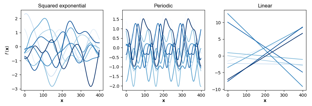
In my mind, Figure $1$ makes clear that the kernel is a kind of prior or inductive bias. Given the same data, different kernels specify completely different functions. See A2 for the abbreviated code to generate this figure.

Prediction

Ultimately, we are interested in prediction or generalization to unseen test data given training data. Intuitively, what this means is that we do not want just any functions sampled from our prior; rather, we want functions that “agree” with our training data (Figure $2$).

Figure 2: Ten samples from a GP with a squared exponential kernel and four noise-free observations. A conditional Gaussian distribution has $0$ variance at the observed data points.

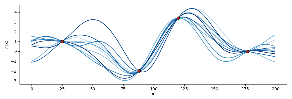
There is an elegant solution to this modeling challenge: conditionally Gaussian random variables. Recall that a GP is actually an infinite-dimensional object, while we only compute over finitely many dimensions. This means the the model of the concatenation of $\mathbf{f}$ and $\mathbf{f}_{*}$ is

$\begin{bmatrix} \mathbf{f}_* \\ \mathbf{f} \end{bmatrix} \sim \mathcal{N} \Bigg( \begin{bmatrix} \mathbf{0} \\ \mathbf{0} \end{bmatrix}, \begin{bmatrix} K(\mathbf{X}_{*}, \mathbf{X}_{*}) & K(\mathbf{X}_{*}, \mathbf{X}) \\ K(\mathbf{X}, \mathbf{X}_{*}) & K(\mathbf{X}, \mathbf{X}) \end{bmatrix} \Bigg) \tag{5}$

where for ease of notation, we assume $m(\cdot) = \mathbf{0}$. Using basic properties of multivariate Gaussian distributions (see A3), we can compute

$\begin{aligned} \mathbf{f}_{*} \mid \mathbf{f} \sim \mathcal{N}(&K(\mathbf{X}_{*}, \mathbf{X}) K(\mathbf{X}, \mathbf{X})^{-1} \mathbf{f},\\ &K(\mathbf{X}_*, \mathbf{X}_*) - K(\mathbf{X}_*, \mathbf{X}) K(\mathbf{X}, \mathbf{X})^{-1} K(\mathbf{X}, \mathbf{X}_*)). \end{aligned} \tag{6}$

While we are still sampling random functions $\mathbf{f}_{*}$, these functions “agree” with the training data. To see why, consider the scenario when $\mathbf{X}_{*} = \mathbf{X}$; the mean and variance in Equation $6$ are

$\begin{aligned} K(\mathbf{X}, \mathbf{X}) K(\mathbf{X}, \mathbf{X})^{-1} \mathbf{f} &\qquad \rightarrow \qquad \mathbf{f} \\ K(\mathbf{X}, \mathbf{X}) - K(\mathbf{X}, \mathbf{X}) K(\mathbf{X}, \mathbf{X})^{-1} K(\mathbf{X}, \mathbf{X})) &\qquad \rightarrow \qquad \mathbf{0}. \end{aligned}$

In other words, the variance at the training data points is $\mathbf{0}$ (non-random) and therefore the random samples are exactly our observations $\mathbf{f}$.

See A4 for the abbreviated code to fit a GP regressor with a squared exponential kernel. This code will sometimes fail on matrix inversion, but this is a technical rather than conceptual detail for us. Rasmussen and Williams (and others) mention using a Cholesky decomposition, but this is beyond the scope of this post.

Noisy observations

In Figure $2$, we assumed each observation was noiseless—that our measurements of some phenomenon were perfect—and fit it exactly. But in practice, we might want to model noisy observations,

$y = f(\mathbf{x}) + \varepsilon$

where $\varepsilon$ is i.i.d. Gaussian noise or $\varepsilon \sim \mathcal{N}(0, \sigma^2)$. Then Equation $5$ becomes

$\begin{bmatrix} \mathbf{f}_* \\ \mathbf{f} \end{bmatrix} \sim \mathcal{N} \Bigg( \begin{bmatrix} \mathbf{0} \\ \mathbf{0} \end{bmatrix}, \begin{bmatrix} K(\mathbf{X}_{*}, \mathbf{X}_{*}) & K(\mathbf{X}_{*}, \mathbf{X}) \\ K(\mathbf{X}, \mathbf{X}_{*}) & K(\mathbf{X}, \mathbf{X}) + \sigma^2 \mathbf{I} \end{bmatrix} \Bigg)$

while Equation $6$ becomes

$\begin{aligned} \mathbf{f}_{*} \mid \mathbf{y} &\sim \mathcal{N}(\mathbb{E}[\mathbf{f}_{*}], \text{Cov}(\mathbf{f}_{*})) \end{aligned}$

where

$\begin{aligned} \mathbb{E}[\mathbf{f}_{*}] &= K(\mathbf{X}_{*}, \mathbf{X}) [K(\mathbf{X}, \mathbf{X}) + \sigma^2 \mathbf{I}]^{-1} \mathbf{y} \\ \text{Cov}(\mathbf{f}_{*}) &= K(\mathbf{X}_{*}, \mathbf{X}_{*}) - K(\mathbf{X}_{*}, \mathbf{X}) [K(\mathbf{X}, \mathbf{X}) + \sigma^2 \mathbf{I}]^{-1} K(\mathbf{X}, \mathbf{X}_{*})) \end{aligned} \tag{7}$

Mathematically, the diagonal noise adds “jitter” to so that $k(\mathbf{x}_n, \mathbf{x}_n) \neq 0$. In other words, the variance for the training data is greater than $0$. The reader is encouraged to modify the code to fit a GP regressor to include this noise.

Uncertainty

An important property of Gaussian processes is that they explicitly model uncertainty or the variance associated with an observation. This is because the diagonal of the covariance matrix captures the variance for each data point. This diagonal is, of course, defined by the kernel function. For example, the squared exponential is clearly $1$ when $\mathbf{x}_n = \mathbf{x}_m$, while the periodic kernel’s diagonal depends on the parameter $\sigma_p^2$. However, recall that the variance of the conditional Gaussian decreases around the training data, meaning the uncertainty is clamped, speaking visually, around our observations.

Figure 3: A visualization of twice the standard deviation ($95\%$ confidence interval) of a GP fit to (left) $4$, (middle) $12$, and (right) $24$ samples. As the number of samples increases, the model's uncertainty decreases, and this uncertainty-reduction is quantified by a decrease in a conditional Gaussian's variance.

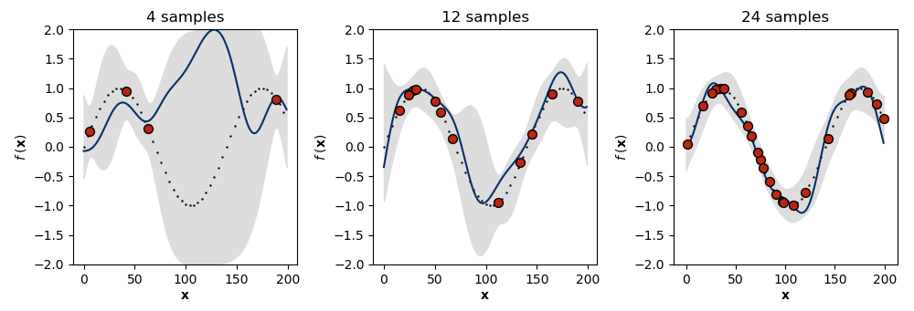
One way to understand this is to visualize two times the standard deviation ($95\%$ confidence interval) of a GP fit to more and more data from the same generative process (Figure $3$). We can see that in the absence of much data (left), the GP falls back on its prior, and the model’s uncertainty is high. However, as the number of observations increases (middle, right), the model’s uncertainty in its predictions decreases. If we modeled noisy observations, then the uncertainty around the training data would also be greater than $0$ and could be controlled by the hyperparameter $\sigma^2$. See A5 for the abbreviated code required to generate Figure $3$.

Conclusion

There is a lot more to Gaussian processes. I did not discuss the mean function or hyperparameters in detail; there is GP classification (Rasmussen & Williams, 2006), inducing points for computational efficiency (Snelson & Ghahramani, 2006), and a latent variable interpretation for high-dimensional data (Lawrence, 2004), to mention a few. However, a fundamental challenge with Gaussian processes is scalability, and it is my understanding that this is what hinders their wider adoption. Exact inference is hard because we must invert a covariance matrix whose sizes increases quadratically with the size of our data, and that operation (matrix inversion) has complexity $O(N^3)$. At present, the state of the art is still on the order of a million data points (Wang et al., 2019).

Appendix

A1: Simplifying the mean vector and covariance matrix

First, note

$\begin{aligned} \mathbb{E}[\mathbf{w}] &\triangleq \mathbf{0} \\ \text{Var}(\mathbf{w}) &\triangleq \alpha^{-1} \mathbf{I} = \mathbb{E}[\mathbf{w} \mathbf{w}^{\top}] \\ \mathbb{E}[y_n] &= \mathbb{E}[\mathbf{w}^{\top} \mathbf{x}_n] = \sum_i x_i \mathbb{E}[w_i] = 0 \end{aligned}$

Thus, the mean of $\mathbf{y}$ is

$\mathbb{E}[\mathbf{y}] = \mathbf{\Phi} \mathbb{E}[\mathbf{w}] = \mathbf{0}$

and its covariance is

$\begin{aligned} \text{Cov}(\mathbf{y}) &= \mathbb{E}[(\mathbf{y} - \mathbb{E}[\mathbf{y}])(\mathbf{y} - \mathbb{E}[\mathbf{y}])^{\top}] \\ &= \mathbb{E}[\mathbf{y} \mathbf{y}^{\top}] \\ &= \mathbb{E}[\mathbf{\Phi} \mathbf{w} \mathbf{w}^{\top} \mathbf{\Phi}^{\top}] \\ &= \mathbf{\Phi} \text{Var}(\mathbf{w}) \mathbf{\Phi}^{\top} \\ &= \frac{1}{\alpha} \mathbf{\Phi} \mathbf{\Phi}^{\top} \end{aligned}$

A2: Sampling from a GP prior

Below is abbreviated code—I have removed easy stuff like specifying colors—for Figure $2$:

import numpy as np
import matplotlib.pyplot as plt


def squared_exponential_kernel(x1, x2):
    return np.exp(-1/2. * np.linalg.norm([x1 - x2], 2)**2)

def periodic_kernel(x1, x2):
    p = 3
    return np.exp(-2 * np.sin((np.pi * np.abs([x1 - x2]))/p)**2)

def linear_kernel(x1, x2):
    b = 1; c = 0
    return b + ((x1 - c) * (x2 - c))

def apply_kernel(n, kernel):
    K = np.empty((n, n))
    for i in range(n):
        x1 = X[i]
        for j in range(n):
            x2 = X[j]
            K[i, j] = kernel(x1, x2)
    return K


fig, axes = plt.subplots(1, 3)
cov_funcs = [squared_exponential_kernel, periodic_kernel, linear_kernel]
n_samples = 400
n_priors  = 10
X         = np.linspace(-5, 5, n_samples)

for kernel, ax in zip(cov_funcs, axes):
    mean = np.zeros(n_samples)
    cov  = apply_kernel(n_samples, kernel)
    for _ in range(n_priors+1):
        f = np.random.multivariate_normal(mean, cov)
        ax.plot(np.arange(n_samples), f)

plt.show()

A3: Sampling from a conditionally Gaussian distribution

Let $\mathbf{x}$ and $\mathbf{y}$ be jointly Gaussian random variables such that

$\begin{bmatrix} \mathbf{x} \\ \mathbf{y} \end{bmatrix} \sim \mathcal{N} \Big( \begin{bmatrix} \boldsymbol{\mu}_x \\ \boldsymbol{\mu}_y \end{bmatrix}, \begin{bmatrix} \boldsymbol{\Sigma}_{xx} & \boldsymbol{\Sigma}_{xy} \\ \boldsymbol{\Sigma}_{yx} & \boldsymbol{\Sigma}_{yy} \end{bmatrix} \Big)$

Then the marginal distributions of $\mathbf{x}$ is

$\mathbf{x} \sim \mathcal{N}(\boldsymbol{\mu}_x, \boldsymbol{\Sigma}_{xx}),$

while the conditional distribution is

$\mathbf{x} \mid \mathbf{y} \sim \mathcal{N}(\boldsymbol{\mu}_x + \boldsymbol{\Sigma}_{xy} \boldsymbol{\Sigma}_{yy}^{-1} (\mathbf{y} - \boldsymbol{\mu}_y), \boldsymbol{\Sigma}_{xx} - \boldsymbol{\Sigma}_{xy} \boldsymbol{\Sigma}_{yy}^{-1} \boldsymbol{\Sigma}_{yx})$

This is a common fact that can be either re-derived or found in many textbooks.

A4: Fitting a Gaussian process regression model

The naive (and readable!) implementation for fitting a GP regressor is straightforward. Below is an implementation using the squared exponential kernel, noise-free observations, and NumPy’s default matrix inversion function:

import numpy as np
import matplotlib.pyplot as plt


def kernel(X, Y):
    K = np.empty((len(X), len(Y)))
    for i, x in enumerate(X):
        for j, y in enumerate(Y):
            K[i, j] = np.exp(-1/2. * np.linalg.norm([x - y], 2)**2)
    return K


n_samples = 200
n_train   = 10
gen_fn    = lambda x: np.sin(2 * np.pi * 5 * x / 700)
inds      = np.random.choice(n_samples, n_train)
Y_train   = gen_fn(inds)
X_test    = np.linspace(-5, 5, n_samples)
X_train   = X_test[inds]

K_st = kernel(X_test,  X_train)
K_tt = kernel(X_train, X_train)
K_ss = kernel(X_test,  X_test)
K_ts = kernel(X_train, X_test)

mean = K_st @ np.linalg.inv(K_tt) @ Y_train
cov  = K_ss - (K_st @ np.linalg.inv(K_tt) @ K_ts)

y_pred = np.random.multivariate_normal(mean, cov)
plt.plot(np.arange(n_samples), y_pred)
plt.scatter(inds, Y_train)
plt.show()

A5: Modeling uncertainty

Below is code for plotting the uncertainty modeled by a Gaussian process for an increasing number of data points:

import numpy as np
import matplotlib.pyplot as plt


def kernel(X, Y):
    kern = lambda x, y: np.exp(-1/2. * np.linalg.norm([x - y], 2)**2)
    K = np.empty((len(X), len(Y)))
    for i, x in enumerate(X):
        for j, y in enumerate(Y):
        K[i, j] = kern(x, y)
    return K

def gen_fn(x):
    return np.sin(2 * np.pi * 5 * x / 700)

def get_data(n_samples, n_train):
    inds = []
    while len(inds) < n_train:
        r = np.random.randint(n_samples)
        if r not in inds:
        inds.append(r)
    X_train_inds = np.array(inds)
    Y_train      = gen_fn(X_train_inds)
    X_test       = np.linspace(-5, 5, n_samples)
    X_train      = X_test[X_train_inds]
    return X_train_inds, Y_train, X_test, X_train


fig, axes = plt.subplots(1, 3)
n_samples = 200

for ax, n_train in zip(axes.flat, [4, 12, 24]):
    X_train_inds, Y_train, X_test, X_train = get_data(n_samples, n_train)

    K_st = kernel(X_test,  X_train)
    K_tt = kernel(X_train, X_train)
    K_ss = kernel(X_test,  X_test)
    K_ts = kernel(X_train, X_test)
    
    noise = np.eye(KXX.shape[0]) * 0.05
    mean = K_st @ np.linalg.inv(K_tt + noise) @ Y_train
    cov  = K_ss - (K_st @ np.linalg.inv(K_tt + noise) @ K_ts)

    f_test = np.random.multivariate_normal(mean, cov)
    ax.plot(np.arange(n_samples), f_test)
    std = np.sqrt(np.diag(cov))
    ax.fill_between(np.arange(n_samples), mean-2*std, mean+2*std)
    ax.scatter(X_train_inds, Y_train)

    x = np.arange(0, n_samples, 4)
    ax.scatter(x, gen_fn(x))

plt.show()