Laplace's Method

The motivation for Laplace’s method (Laplace, 1774) is more general than our goal of density estimation, and it is worth exploring. Suppose we want to approximate an integral of the form

$\int_a^b e^{k f(x)} \text{d}x \tag{1}$

where $f(x)$ is a twice differentiable function with a global maximum at $x_0$, $k > 0$ and is ideally large, and the endpoints $a$ and $b$ can be infinite. Consider this ratio,

$\frac{e^{k f(x_0)}}{e^{k f(x)}} = e^{k(f(x_0) - f(x))}$

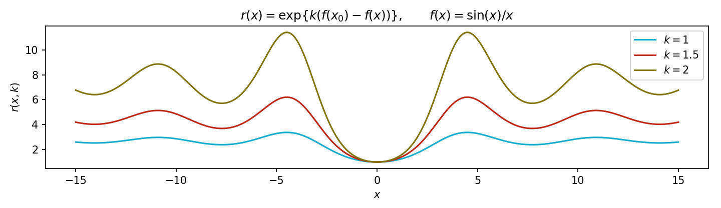
which increases exponentially as $k$ increases linearly. So for large $k$, the difference between the maximum point and the rest of the function is accentuated (Figure $1$).

Figure 1: Let $f(x) = \sin(x)/x$. Then $x_0 = 0$ and $\lim_{x \rightarrow x_0} f(x) = 1$. As $k$ increases, the ratio $r(x) = \exp\{k(f(x_0) - f(x))\}$ increases exponentially.

This observation about the behavior of $e^{k f(x)}$ is what motivates Laplace’s method, and it suggests that we can approximate $f(x)$ using a Taylor expansion around $x_0$,

$f(x) = f(x_0) + \frac{f^{\prime}(x_0)}{1!} (x - x_0) + \frac{f^{\prime\prime}(x_0)}{2!} (x - x_0)^2 + \dots.$

Since $x_0$ is at a maximum, $f^{\prime}(x_0) = 0$, and the first-order term disappears. If we drop the higher-order terms, then

$f(x) \approx f(x_0) + \frac{1}{2} f^{\prime\prime}(x_0) (x - x_0)^2 \tag{2}$

As an example, consider the function $f(x) = \sin(x)/x$ from Figure $1$. Then we have

$\begin{aligned} f(x) &= \sin(x)/x \\ x_0 &= 0 \\ \lim_{x \rightarrow x_0} f(x) &= 1 \\ \lim_{x \rightarrow x_0} f^{\prime\prime}(x) &= - \frac{1}{3} \\ &\Downarrow \\ \exp\Big\{k \Big(\frac{\sin(x)}{x}\Big)\Big\} &\approx \exp\Big\{ k \Big(1 - \frac{1}{6} x^2\Big)\Big\} \end{aligned}$

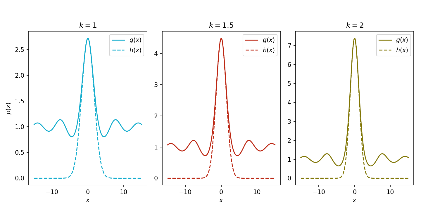
Figure $2$ shows the function $e^{k f(x)}$ and the approximation for varying values of $k$. This captures our earlier point, which is that as $k$ increases, the function $e^{k f(x)}$ becomes more peaked around $x_0$, and thus our Taylor-expanded approximation improves.

Figure 2: Let $f(x) = \sin(x)/x$, $g(x) = e^{k f(x)}$, and $h(x) = \exp\Big(f(x_0) + \frac{f^{\prime\prime}(x_0)}{2} (x - x_0)^2 \Big)$. The panels compare $g(x)$ to its approximation $h(x)$ for $k \in \{1, 1.5, 2\}$.

At this point, you might have already noticed that our approximation (Equation $2$), if appropriately normalized, is just the Gaussian PDF centered at $x_0$. Since $x_0$ is a maximum, $f^{\prime\prime}(x_0) < 0$ (recall the Second Derivative Test) and thus $f^{\prime\prime}(x_0) = -\|f^{\prime\prime}(x_0)\|$. We can approximate Equation $1$ as,

$\begin{aligned} \int_a^b e^{k f(x)} \text{d}x &\approx \int_a^b \exp\Big\{ k \Big( f(x_0) - \frac{1}{2}|f^{\prime\prime}(x_0)|(x - x_0)^2 \Big) \Big\} \text{d}x \\ &= e^{k f(x_0)} \int_a^b \exp\Big\{ - \frac{1}{2} k |f^{\prime\prime}(x_0)|(x - x_0)^2 \Big\} \text{d}x \end{aligned}$

This is a Gaussian integral if $a = -\infty$ and $b = \infty$, and is a Gaussian density if appropriately normalized. This is precisely what motivates Laplace’s method for density approximation.

Density approximation

Now consider the goal of approximating a distribution, ideally unimodal, with a Gaussian. Now our unnormalized density is $f(x)$, and the normalized density is $p(x) = \frac{1}{Z} f(x)$ where $Z$ is unknown. The mode or peak of this distribution occurs at the maximum $x_0$.

Let’s Taylor-expand $\ln f(x)$ around the point $x_0$. If we write the negative of the second derivative in the second-order term as $A$ and drop the higher-order terms, then

$\ln f(x) \approx \ln f(x_0) - \frac{A}{2} (x - x_0)^2, \qquad A = -\frac{\partial^2}{\partial x^2} \ln f(x) \Big|_{x = x_0} \tag{3}$

If we are estimating parameters, then $x_0$ is just the maximum likelihood or maximum a posteriori (MAP) estimate, and $A$ is just the negative log likelihood evaluated at the optimal parameter. Thus, we can approximate $p(x)$ with an unnormalized density $q^{*}(x)$ such that,

$q^{*}(x) \triangleq f(x_0) \exp \Big\{ - \frac{A}{2} (x - x_0)^2 \Big\}$

Since we assume $q^{*}(x)$ is Gaussian, $A = 1 / \sigma^2$, and the normalizing constant is

$Z_q \triangleq \sqrt{2 \pi} f(x_0) \frac{1}{\sqrt{A}}$

Putting it together, the normalized density $q(x)$ is

$p(x) \approx q(x) = \frac{q^{*}(x)}{Z_q} = \sqrt{\frac{A}{2 \pi}} \exp \Big\{ - \frac{A}{2} (x - x_0)^2 \Big\}.$

Notice that in density estimation, $k$ is not free parameter because we want our integral to integrate to $1$.

We can generalize Laplace’s method to a $p$-dimensional Gaussian random vector $\mathbf{x}$. Let the constant $A$ from the previous section be a Hessian matrix $\mathbf{A}$ such that

$A_{ij} = - \frac{\partial^2}{\partial x_i \partial x_j} \ln f(\mathbf{x}) \Big|_{\mathbf{x} = \mathbf{x}_0}.$

Then the approximation in Equation $3$ is

$\ln f(x) \approx \ln f(\mathbf{x}_0) - \frac{1}{2} (\mathbf{x} - \mathbf{x}_0)^{\top} \mathbf{A}^{-1} (\mathbf{x} - \mathbf{x}_0).$

and the normalizing constant is

$Z_q \triangleq \sqrt{2 \pi} f(\mathbf{x}_0) \frac{1}{\sqrt{\mathbf{\det(A)}}}.$

This is derived from the standard form a multivariate Gaussian with $\mathbf{A}$ in place of the covariance matrix $\boldsymbol{\Sigma}$. The normalized density is

$p(\mathbf{x}) \approx q(\mathbf{\mathbf{x}}) = \frac{q^{*}(x)}{Z_q} = \sqrt{\frac{\mathbf{\det(A)}}{2 \pi}} \exp \Big\{ - \frac{1}{2} (\mathbf{x} - \mathbf{x}_0)^{\top} \mathbf{A}^{-1} (\mathbf{x} - \mathbf{x}_0) \Big\}.$

Thus, we have seen that Laplace’s method places a Gaussian at the mode of the approximated distribution and matches the curvature of the density around that point.

MacKay’s exercise

As a complete example, let’s work through David MacKay’s exercise 27.1, part (a):

A photon counter is pointed at a remote star for one minute, in order to infer the rate of photons arriving at the counter per minute, $\lambda$. Assuming the number of photons collected $r$ has a Poisson distribution with mean $\lambda$,

$P(r \mid \lambda) = \exp(-\lambda) \frac{\lambda^r}{r!},$

and assuming the improper prior $P(\lambda) = 1 / \lambda$, make Laplace approximations to the posterior distribution over $\lambda$.

First, since we have a prior, note that $\lambda_0 = \lambda_{\text{MAP}}$. The posterior is

$p(\lambda \mid r) \propto p(r \mid \lambda) p(\lambda) = \frac{e^{-\lambda} \lambda^{r-1}}{r!}$

The negative log of the posterior is

$\begin{aligned} Q &= - \ln p(\lambda \mid r) \\ &= - [ \ln(e^{-\lambda}) + \ln(\lambda^{r-1}) - \ln(r!)] \\ &\propto \lambda - (r - 1) \log(\lambda) \end{aligned}$

We drop the term $\ln(r!)$ because it is just a constant with respect to $\lambda_{\text{MAP}}$. Now let’s find $\lambda_{\text{MAP}}$:

$\begin{aligned} \frac{\partial Q}{\partial \lambda} &= 1 - \frac{r-1}{\lambda} \\ 0 &= 1 - \frac{r-1}{\lambda} \\ \lambda_{\text{MAP}} &= r - 1 \end{aligned}$

Next, we compute the second derivative, evaluated at the mode of the distribution,

$A = \frac{\partial^2 Q}{\partial \lambda^2} \Bigg|_{\lambda = \lambda_{\text{MAP}}} = \frac{r-1}{\lambda^2_{\text{MAP}}} = \frac{r - 1}{(r-1)^2} = \frac{1}{r - 1}$

Since $A = \frac{1}{r - 1}$ and $\lambda_{\text{MAP}} = r - 1$, the normalized density is

$\begin{aligned} q(\lambda) &= \sqrt{\frac{A}{2 \pi}} \exp \Big\{ - \frac{A}{2} (\lambda - \lambda_{\text{MAP}})^2 \Big\} \\ &= \frac{1}{\sqrt{2 \pi (r - 1)}} \exp \Big\{ - \frac{1}{2 (r - 1)} (\lambda - (r - 1))^2 \Big\} \end{aligned}$

This is a Gaussian with a mean and variance of $r - 1$,

$\boxed{p(\lambda \mid r) \approx \mathcal{N}(\lambda; r - 1, r - 1)}$

and we’re done.

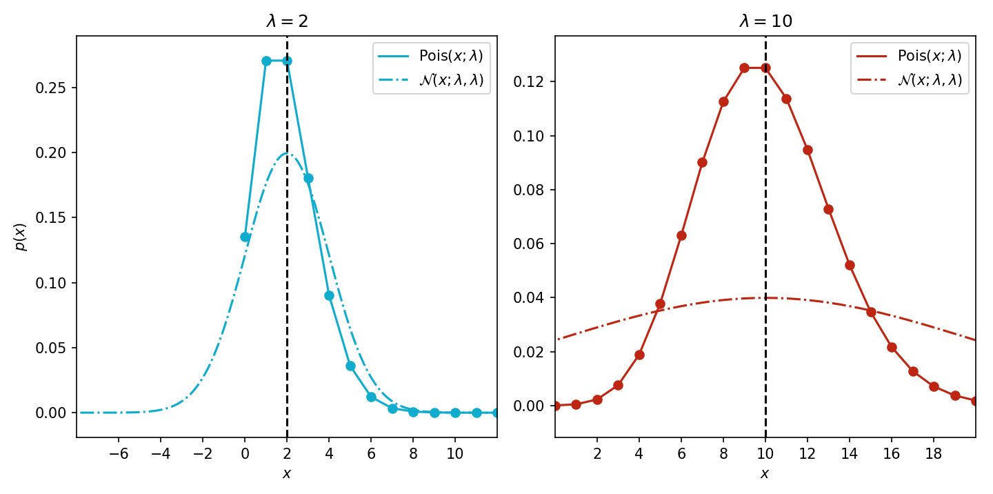
As a final warning, observe that a Gaussian approximation is often suboptimal. For example, we just derived a Gaussian distribution that has an identical mean and variance. For ease of visualization, let’s recalculate our Laplace approximation of just the Poisson distribution without the improper prior from MacKay. We can see that the approximation gets worse as $\lambda$ gets bigger (Figure $3$).

Figure 3: Laplace approximations of $\text{Pois}(x \mid \lambda)$ for $\lambda \in \{2, 10\}$. Since each Gaussian approximation has both a mean and a variance that are functions of $\lambda$, the variance of the Gaussian approximation quickly blows up when $\lambda$ is large.

This is due to the fact that the Gaussian approximation has both a mean and a variance of $\lambda$, and its spread increases faster than the Poisson distribution’s.