Randomized Singular Value Decomposition

1. Introduction

Many standard algorithms for dealing with matrices, such as matrix multiplication and low-rank matrix approximation, are expensive or intractable in large-scale machine learning and statistics. For example, given an $m \times n$ matrix $\textbf{A}$ where both $m$ and $n$ are large, a method such as singular value decomposition (SVD) will require memory and time which is superlinear in $m$ and $n$ (Drineas et al., 2006).

A growing area of research, randomized numerical linear algebra (RandNLA), combines probability theory with numerical linear algebra to develop fast, randomized algorithms with theoretical guarantees that such algorithms are, in some sense, a good approximation of some full computation (Drineas & Mahoney, 2016) (Mahoney, 2016). The main insight is that randomness is an algorithmic resource creating efficient, unbiased approximations of nonrandom operations.

A seminal paper in RandNLA, “Finding structure with randomness: Probabilistic algorithms for constructing approximate matrix decompositions” by Halko, Martinsson, and Tropp (Halko et al., 2011), demonstrated that a modular framework could be used for randomized matrix approximations. The goal of this post is to deeply understand this paper, with a particular focus on randomized SVD. I present Halko et al’s modular framework through the randomized SVD algorithm, walk the reader through a few theoretical results, and reproduce a couple numerical experiments.

This post is organized as follows. In Section 2, I introduce randomized SVD through the lens of Halko et al’s general framework for low-rank matrix approximations. This motivates Section 2.2, in which I discuss randomized range finders. These are the probabilistic crux of the paper. Sections 2.3–2.5 cover theory and algorithmic improvements. In Section 3, I discuss the key numerical results of the paper and demonstrate that I am able to both implement randomized SVD and reproduce these results.

2. Randomized SVD

2.1. Two-stage framework

Consider the general problem of low-rank matrix approximation. Given an $m \times n$ matrix $\textbf{A}$, we want $m \times k$ and $k \times n$ matrices $\textbf{B}$ and $\textbf{C}$ such that $k \ll n$ and $\textbf{A} \approx \textbf{B} \textbf{C}$. To approximate this computation using randomized algorithms, Halko et al propose a two-stage computation:

• Step 1: Compute an approximate basis for the range of $\textbf{A}$. We want a matrix $\textbf{Q}$ with $\ell$ orthonormal columns ($k \leq \ell \leq n$) that captures the action of $\textbf{A}$. Formally, $\textbf{A} \approx \textbf{Q} \textbf{Q}^{*} \textbf{A}$.

• Step 2: Given such a matrix $\textbf{Q}$—which is much smaller than $\textbf{A}$—use it to compute our desired matrix factorization.

In the case of SVD, imagine we had access to $\textbf{Q}$. Then randomized SVD is the following:

Algorithm 1. Randomized SVD

Given an orthonormal matrix $\textbf{Q}$ s.t. $\textbf{A} \approx \textbf{Q} \textbf{Q}^{*} \textbf{A}:$

• Form $\textbf{B} = \textbf{Q}^{*} \textbf{A}$
• Compute the SVD of $\textbf{B}$, i.e. $\textbf{B} = \tilde{\textbf{U}} \boldsymbol{\Sigma} \textbf{V}^{*}$
• Set $\textbf{U} = \textbf{Q} \tilde{\textbf{U}}$.
• Return $\textbf{U}, \boldsymbol{\Sigma}, \textbf{V}^{*}$

The efficiency of this algorithm comes from $\textbf{B}$ being small relative to $\textbf{A}$. Since $\textbf{A} \approx \textbf{Q} \textbf{Q}^{*} \textbf{A} = \textbf{Q} (\tilde{\textbf{U}} \boldsymbol{\Sigma} \textbf{V}^{*})$, setting $\textbf{U} = \textbf{Q} \tilde{\textbf{U}}$ produces a low-rank approximation, $\textbf{A} \approx \textbf{U} \boldsymbol{\Sigma} \textbf{V}^{*}$.

Note that randomness only occurs in Step 1 and that Step 2 is deterministic given $\textbf{Q}$. Thus, the algorithmic challenge is to efficiently compute $\textbf{Q}$ through randomized methods. Halko et al present several algorithms to do this, called randomized range finders.

2.2. Randomized range finders

The goal of a randomized range finder is to produce an orthonormal matrix $\textbf{Q}$ with as few columns as possible such that

$\lVert (\textbf{I} - \textbf{Q}\textbf{Q}^{*} \textbf{A}) \rVert \leq \varepsilon \tag{1}$

for some desired tolerance $\varepsilon$.

Halko et al’s solution is motivated by Johnson and Lindenstrauss’s seminal paper (Johnson & Lindenstrauss, 1984) that showed that pairwise distances among a set of points in a Euclidean space are roughly maintained when projected into a lower-dimensional Euclidean space. The basic idea is to draw $\ell$ Gaussian random vectors, $\boldsymbol{\omega}^{(1)}, \boldsymbol{\omega}^{(2)}, \dots \boldsymbol{\omega}^{(l)}$ and project them using the linear map $\textbf{A}$. Intuitively, we are randomly sampling the range of $\textbf{A}$. And finding an orthonormal basis for these vectors gives us our desired $\textbf{Q}$. This scheme is formally described in Algorithm 2.

Algorithm 2: Randomized range finder

Let $\ell$ be a sampling parameter indicating the number of Gaussian random vectors to draw for $\boldsymbol{\boldsymbol{\Omega}}$.

• Draw an $n \times \ell$ Gaussian random matrix $\boldsymbol{\boldsymbol{\Omega}}$
• Generate an $m \times \ell$ matrix $\textbf{Y} = \textbf{A} \boldsymbol{\boldsymbol{\Omega}}$
• Generate an orthonormal matrix $\textbf{Q}$, e.g. using QR factorization $\textbf{Y} = \textbf{Q} \textbf{R}$.

Note that Algorithm 2 takes as input a sampling parameter $\ell$ where $\ell \geq k$ ideally. Then $p = \ell - k$ is the oversampling parameter. In their Section 4.2, Halko et al claim:

For Gaussian test matrices, it is adequate to choose the oversampling parameter to be a small constant, such as $p = 5$ or $p = 10$. There is rarely any advantage to select $p > k$.

Justification for this claim can be found in Section 10.2 of their paper. For completeness, I provide one theoretical result in Section 2.3. But the main result is that with just a few more samples than true rank of $\textbf{A}$, we can get an approximation with an error that is close to the theoretical minimum.

A useful modification to Algorithm 2 is the ability to automatically select $\ell$ based on the acceptable error or tolerance $\varepsilon$. The main idea is that the orthonormal basis $\textbf{Q}$ can be constructed incrementally, and we can stop when the error is acceptable. Let $\textbf{Q}^{(i)}$ denote an iteration of the $\textbf{Q}$ matrix with $i$ columns. Then the empty basis matrix is $\textbf{Q}^{(0)}$. Algorithm 3 incrementally generates $\textbf{Q}$.

Algorithm 3: Iterative construction of $\textbf{Q}$

• Draw an $n \times 1$ Gaussian random vector, $\boldsymbol{\omega}^{(i)}$, and set $\textbf{y}^{(i)} = A \boldsymbol{\omega}^{(i)}$.
• Construct $\tilde{\textbf{q}} = \big(\textbf{I} - \textbf{Q}^{(i-1)} (\textbf{Q}^{(i-1)})^{*} \big) \textbf{y}^{(i)}$
• Set $\textbf{q}^{(i)} = \tilde{\textbf{q}^{(i)}} / \lVert \tilde{\textbf{q}^{(i)}} \rVert$
• Form $\textbf{Q}^{(i)} = [\textbf{Q}^{(i-1)} \textbf{q}^{(i)}]$

This procedure is reminiscent of the Gram–Schmidt process (Björck, 1994). If we integrate this iterative procedure into Algorithm 2, we get Halko et al’s adaptive randomized range finder in their Section 4.4.

2.3. Performance Analysis

Halko et al present a number of theoretical results for their algorithms, but one illustrative result is their Theorem 1.1. As a preliminary, note Equation $2$ per (Mirsky, 1960), which claims that the theoretical minimum of any low-rank matrix approximation of $\textbf{A}$ is equal to the $(j+1)$th singular value:

$\min_{\text{rank}(\textbf{X}) \leq j} \lVert \textbf{A} - \textbf{X} \rVert = \sigma_{j+1}. \tag{2}$

Given this, consider their Theorem 1.1:

Theorem 1.1

Suppose that $\textbf{A}$ is a real $m \times n$ matrix. Select a target rank $k \geq 2$ and an oversampling parameter $p \geq 2$, where $k + p \leq \min\{m, n\}$. Execute the proto-algorithm with a standard Gaussian test matrix to obtain an $m \times (k+p)$ matrix $\textbf{Q}$ with orthonormal columns. Then

$> \mathbb{E} \lVert \textbf{A} - \textbf{Q} \textbf{Q}^{*} \textbf{A} \rVert \leq \Big[ 1 + \frac{4 \sqrt{k + p}}{p - 1} \cdot \sqrt{\min\{m, n\}} \Big] \sigma_{k+1} >$

where $\mathbb{E}$ denotes the expectation with respect to the random test matrix and $\sigma_{k+1}$ is the $(k+1)$th singular value of $\textbf{A}$.

For a proof, see Halko et al’s proof of Theorem 10.6, which generalizes Theorem 1.1 above.

What this theorem states is that their randomized range finder produces a $\textbf{Q}$ with an error that is within a small polynomial factor of the theoretical minimum (Equation $2$). In other words, if $m$, $n$, and $k$ are all fixed parameters of $\textbf{A}$, what matters is its singular spectrum.

It makes intuitive sense that the quality of any randomized approximation of $\textbf{A}$ depends on the structure of $\textbf{A}$. If $\textbf{A}$ is full-rank or if its singular spectrum decays slowly, there is only so well that a randomized low-rank technique can do.

2.6. Subspace iteration

As discussed in Section 2.4, when the singular spectrum of $\textbf{A}$ decays slowly, randomized SVD can have high reconstruction error. In this scenario, Halko et al propose taking a couple power iterations (their Algorithm 4.4). The main idea is that power iterations do not modify the singular vectors, but they do reduce the relative weight of small singular values. This forces the spectrum of our approximate range, $\textbf{Y}$, to decay more rapidly.

Formally, if the singular values of $\textbf{A}$ are $\boldsymbol{\Sigma}$, the singular values of $(\textbf{A} \textbf{A}^{*})^{q} \textbf{A}$ are $\boldsymbol{\Sigma}^{2 q + 1}$. This is easy to show. Let $\textbf{A} = \textbf{U} \boldsymbol{\Sigma} \textbf{V}^{*}$. Then

$\begin{aligned} (\textbf{A} \textbf{A}^{*})^q \textbf{A} &= ((\textbf{U} \boldsymbol{\Sigma} \textbf{V}^{*}) (\textbf{U} \boldsymbol{\Sigma} \textbf{V}^{*})^{*})^q \textbf{A} \\ &= (\textbf{U} \boldsymbol{\Sigma} \textbf{V}^{*} \textbf{V} \boldsymbol{\Sigma} \textbf{U}^{*})^q \textbf{A} \\ &= (\textbf{U} \boldsymbol{\Sigma}^2 \textbf{U}^{*})^q \textbf{A}. \end{aligned}$

In other words, the spectrum decays exponentially with the number of power iterations. Since the SVD of $(\textbf{A} \textbf{A}^{*})^q \textbf{A}$ is $\textbf{U} \boldsymbol{\Sigma}^{2q+1} \textbf{V}^{*}$ and since the SVD is unique (Trefethen & Bau III, 1997), the singular vectors are the same.

2.5. Special matrices

In their Sections 5.1-5.4, Halko et al discuss randomized matrix factorizations when $\textbf{A}$ is a special matrix. As a taste for this section, I present the scenario in which $\textbf{A}$ is Hermitian, i.e. when $\textbf{A} = \textbf{A}^{*}$. In this case, $\textbf{A}$ is symmetric and the columns of $\textbf{Q}$ are a basis for both the column and row spaces. Formally, this means:

$\textbf{A} \approx \textbf{Q} \textbf{Q}^{*} \textbf{A} \textbf{Q} \textbf{Q}^{*}$

When Equation $1$ holds, then we have

$\begin{aligned} &\lVert \textbf{A} - \textbf{Q} \textbf{Q}^{*} \textbf{A} \textbf{Q} \textbf{Q}^{*} \rVert \\ &= \lVert \textbf{A} - \textbf{Q} \textbf{Q}^{*} \textbf{A} + \textbf{Q} \textbf{Q}^{*} \textbf{A} - \textbf{Q} \textbf{Q}^{*} \textbf{A} \textbf{Q} \textbf{Q}^{*} \rVert \\ &\leq \lVert \textbf{A} - \textbf{Q} \textbf{Q}^{*} \textbf{A} \rVert + \lVert \textbf{Q} \textbf{Q}^{*}(\textbf{A} - \textbf{A} \textbf{Q} \textbf{Q}^{*}) \rVert \\ &\leq 2 \varepsilon \end{aligned}$

The first inequality is just the triangle inequality. In the second-to-last line, note that the left term is less than $\varepsilon$ by Equation $1$. The second term is also less than $\varepsilon$ because $\lVert \textbf{Q}\textbf{Q}^{*}\rVert = 1$ while

$\lVert \textbf{A} - \textbf{A} \textbf{Q} \textbf{Q}^{*} \rVert = \lVert (\textbf{A} - \textbf{A} \textbf{Q} \textbf{Q}^{*})^{*} \rVert = \lVert \textbf{A} - \textbf{Q} \textbf{Q}^{*} \textbf{A} \rVert$

which relies on the symmetry of $\textbf{A}$. Intuitively, given a Hermitian matrix $\textbf{A}$ and a range approximation $\textbf{Q}$, our error bound is twice the non-Hermitian case because of symmetry, i.e. any element-wise errors are doubled.

Halko et al also analyze the case in which $\textbf{A}$ is positive semidefinite and use Nyström’s method (Drineas & Mahoney, 2005) to efficiently improve standard factorizations, but this discussion is omitted for space.

3. Reproducing numerical results

A major contribution of Halko et al is to demonstrate that their algorithms are not just theoretically elegant but also work in practice. In their Section 7, they present a number of numerical experiments.

A goal of this post was to implement randomized SVD and then demonstrate the correctness of the implementation. The code was written for conceptual clarity and correctness rather than performance. While code written in C, C++, or even FORTRAN (as in Halko et al) might be faster, it is worth observing that my Python code is still performant because the key computational costs, computing the SVD and the matrix-vector product $\textbf{x} \rightarrow \textbf{A} \textbf{x}$, are both done by numpy which has C bindings.

The full code for my implementation of randomized SVD as well as reproducing my results can be found on GitHub.

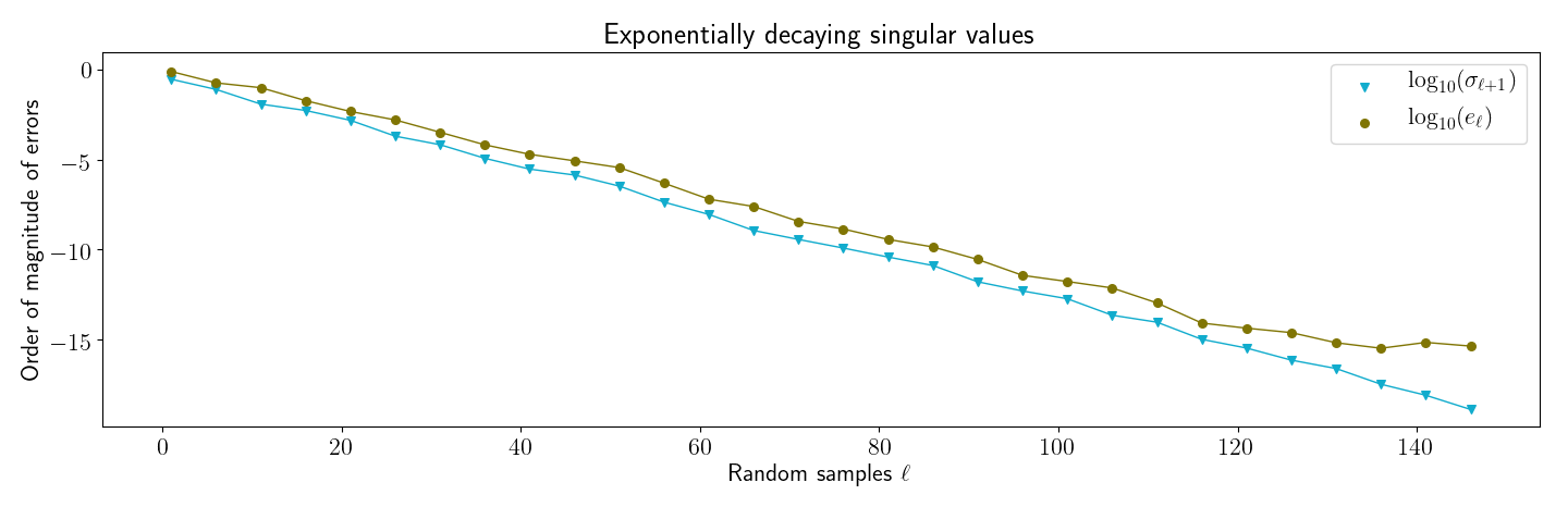
3.1 Decaying singular values

My first reproduction of Halko et al’s numerical results was to reproduce a figure similar to their Figure $7.2$. The idea behind this figure is to show that when the singular spectrum of a matrix $\textbf{A}$ decays, the actual error of randomized SVD on $\textbf{A}$ is close to the theoretical minimum.

First, I generated a matrix with exponentially decaying singular values. This was done by reversing SVD after creating a $\boldsymbol{\Sigma}$ with decreasing values along its diagonal. Then I ran my implementation of randomized SVD over a range of sampling parameter values $\ell \in \{1, 2, \dots 150\}$. For each $\ell$, I computed two values:

• $\sigma_{\ell+1}$: This is the minimum approximation error (Equation $1$).
• $e_{\ell} = \lVert (\textbf{I} - \textbf{Q}^{(\ell)} (\textbf{Q}^{(\ell)})^{*}) \textbf{A} \rVert$: The actual error, computed with np.linalg.norm.

I then generated Figure $1$, which closely matches the main result in Halko et al’s Figure $7.2$. First, note that randomized SVD’s actual error, $e_{\ell}$, is close to the theoretical minimum, $\sigma_{\ell+1}$. Furthermore, as expected, the actual error is always slightly higher than the best we could do.

Figure 1: Demonstration that for a matrix with rapidly decaying singular values, the actual approximation error using randomized SVD approaches but does not go lower than the minimum theoretical approximation error $\sigma_{\ell+1}$. On the $x$-axis, the number of Gaussian random samples $\ell$ varies. On the $y$-axis are the order of magnitudes of the theoretical and actual approximation errors.

3.2 Subspace iterations

My second reproduction of Halko et al’s experiments was to verify that subspace iterations work as predicted. First, I verified my understanding by generating Figure $2$, which plots the singular values for the matrix $(\textbf{A} \textbf{A}^{*})^{q} \textbf{A}$ for varying integers $q$. Clearly, for larger $q$, the singular spectrum decays more rapidly.

Figure 2: Demonstration of subspace iteration on a matrix $\textbf{A}$ with linearly decaying singular values. The index of the singular values of a matrix $(\textbf{A}\textbf{A}^{*})^{q} \textbf{A}$ vary along the $x$-axis. The $y$-axis is the normalized magnitudes of the singular values.

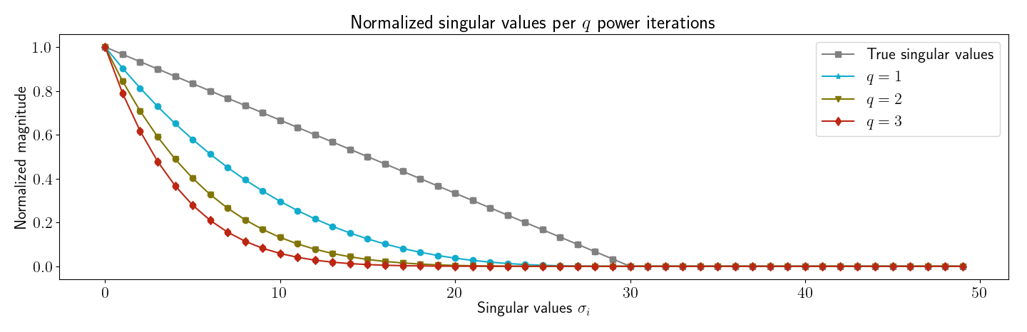
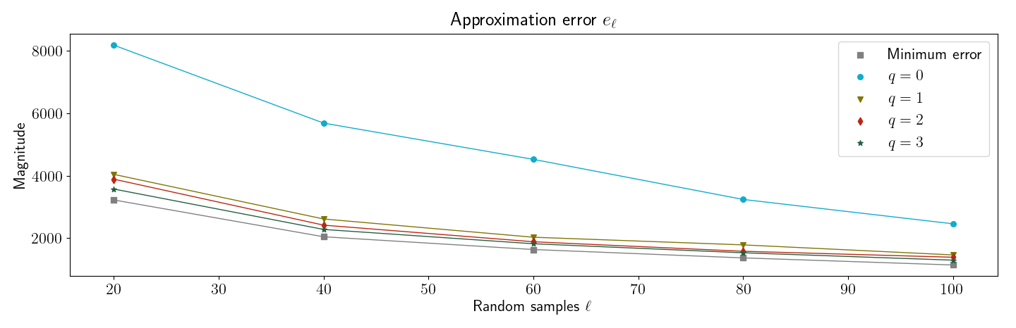
Next, I produced Figure $3$, which is similar to their Figure $7.6$. This simple numerical experiment demonstrates that even when $\textbf{A}$ has slowly decaying singular values—in this case, the singular values decay linearly—subspace iteration can be used to improve the randomized low-rank approximation.

Figure 3: Quantitative demonstration of subspace iteration for a fixed matrix $\textbf{A}$. On the $x$-axis, the number of Gaussian random samples varies. On the $y$-axis, the magnitude of the $\ell_2$ norm between $\textbf{A}$ and its low-rank approximation varies. Each curve represents the number $q$ of subspace iterations.

3.3 Oversampling and accuracy

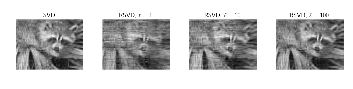
Finally, a common example of the utility of SVD is image reconstruction with the top $k$ singular values for some number $k$. For example, in their Section 7.3, Halko et al discuss measuring the reconstruction error on ``Eigenfaces’’ (Phillips et al., 1998) (Phillips et al., 2000). To qualitatively evaluate the correctness of my implementation as well as the impact of the sampling parameter $\ell$, I generated Figure $4$. This demonstrates that with more Gaussian random samples $\ell$, the reconstruction approaches the true low-rank factorization.

Figure 4: Qualitative demonstration of the sampling parameter $\ell$ for image reconstruction. (Left) A photograph of a raccoon is reconstructed using $k=10$ singular vectors from standard SVD. (Remaining) The same photograph is reconstructed using $k=10$ singular vectors while varying the number of Gaussian random samples $\ell$. As the number of samples increases, the low-rank reconstruction improves.

Conclusion

RandNLA is an exciting area of research that focuses on randomized techniques for numerical linear algebra. Halko, Martinsson, and Tropp’s 2011 paper introduced a two-stage modular framework for computing randomized low-rank matrix factorizations. The work addressed issues such as slowly decaying singular spectrums and special matrices, offered tight bounds on the performance of their algorithms, and provided numerical results demonstrating that these methods work in practice. This post, in addition to providing an overview of the paper, has demonstrated that Halko et al’s work is reproducible and that their theoretical guarantees closely match results from straightforward implementations.

Acknowledgements

Most of the work that went into this post was the result of a class project for ELE 538B at Princeton. I want to thank Yuxin Chen for helpful feedback.