Generalized Least Squares

Ordinary least squares (OLS), when all its assumptions hold, is the best linear unbiased estimator (BLUE). This is the main result of the Gauss–Markov theorem. However, OLS with heteroscedasticity leads to incorrect and inefficient inference. In particular, the $t$-statistics are unreliable, and the estimator is no longer BLUE. See this post for a simple example and code.

However, if we do know the covariance structure of our data, we can use generalized least squares (GLS), developed by Alexander Aitken (Aitkin, 1935). The basic idea of GLS is to normalize our data using the known covariance such that the normalized data adheres to the OLS assumptions. We can then apply the OLS estimator, which is BLUE, to these transformed data.

The goal of this post is to walk through GLS in detail. I’ll present the model, an example, and then prove some basic properties.

Aitken’s generalized least squares

In generalized least squares, we assume the following model:

$\begin{aligned} \mathbf{y} &= \mathbf{X} \boldsymbol{\beta} + \boldsymbol{\varepsilon}, \\ \mathbb{E}[\boldsymbol{\varepsilon} \mid \mathbf{X}] &= \mathbf{0}, \\ \mathbb{V}[\boldsymbol{\varepsilon} \mid \mathbf{X}] &= \sigma^2 \boldsymbol{\Omega} = \boldsymbol{\Sigma}. \end{aligned} \tag{1}$

Here, $\boldsymbol{\Omega}$ is a positive definite matrix, and we assume it is known. This is called generalized least squares because OLS is just a special case of this model, when $\boldsymbol{\Omega} = \mathbf{I}$.

The GLS optimization problem is to minimize the following Gaussian kernel (or Mahalanobis distance):

$\hat{\boldsymbol{\beta}}_{\textsf{GLS}} = \arg\!\min_{\boldsymbol{\beta}} \left\{ (\mathbf{y} - \mathbf{X} \boldsymbol{\beta})^{\top} \boldsymbol{\Omega}^{-1} (\mathbf{y} - \mathbf{X} \boldsymbol{\beta}) \right\}. \tag{2}$

This is different from the OLS optimization problem, which has constant variance which does not effect the optimal coefficients since it can be factored out:

$\hat{\boldsymbol{\beta}}_{\textsf{OLS}} = \arg\!\min_{\boldsymbol{\beta}} \left\{ (\mathbf{y} - \mathbf{X} \boldsymbol{\beta})^{\top} (\mathbf{y} - \mathbf{X} \boldsymbol{\beta}) \right\}. \tag{3}$

Now we could take the gradient of Equation $2$, set it equal to zero, and solve for $\boldsymbol{\beta}_{\textsf{GLS}}$. However, in my mind, there is a simpler way. Instead, simply notice that since $\boldsymbol{\Omega}$ is a positive definite matrix, it has a matrix inverse which a Cholesky decomposition of the form

$\boldsymbol{\Omega}^{-1} = \mathbf{L} \mathbf{L}^{\top}. \tag{4}$

And we can rewrite the Gaussian kernel in Equation $2$ as

$\begin{aligned} &(\mathbf{y} - \mathbf{X} \boldsymbol{\beta})^{\top} \boldsymbol{\Omega}^{-1} (\mathbf{y} - \mathbf{X} \boldsymbol{\beta}) \\ &= (\mathbf{y} - \mathbf{X} \boldsymbol{\beta})^{\top} \mathbf{L} \mathbf{L}^{\top} (\mathbf{y} - \mathbf{X} \boldsymbol{\beta}) \\ &= (\mathbf{L}^{\top} \mathbf{y} - \mathbf{L}^{\top} \mathbf{X} \boldsymbol{\beta})^{\top} (\mathbf{L}^{\top} \mathbf{y} - \mathbf{L}^{\top} \mathbf{X} \boldsymbol{\beta}). \end{aligned} \tag{5}$

In other words, the objective with transformed data $\mathbf{L}^{\top} \mathbf{y}$ and $\mathbf{L}^{\top} \mathbf{X}$ is just the OLS objective, and the transformed errors are homoscedastic,

$\begin{aligned} \mathbb{E}[\mathbf{L}^{\top} \boldsymbol{\varepsilon} \boldsymbol{\varepsilon}^{\top} \mathbf{L} \mid \mathbf{L}^{\top} \mathbf{X}] &= \mathbf{L}^{\top} \mathbb{E}[\boldsymbol{\varepsilon} \boldsymbol{\varepsilon}^{\top} \mid \mathbf{L}^{\top} \mathbf{X}] \mathbf{L} \\ &= \mathbf{L}^{\top} \left( \sigma^2 \boldsymbol{\Omega} \right) \mathbf{L} \\ &= \sigma^2 \mathbf{I}. \end{aligned} \tag{6}$

Why does this work? Since the univariate analog to $\boldsymbol{\Sigma}$ is $\sigma^2$, then $\mathbf{L}^{\top}$ is the multivariate analog to $1 / \sigma$. In other words, $\mathbf{L}^{\top}$ represents a linear transformation to our data such that the new data’s variance is normalized.

Furthermore, note that $\mathbf{L}^{\top} \mathbf{y}$ and $\mathbf{L}^{\top} \mathbf{X}$ adhere to the standard assumptions of OLS: $\mathbf{L}^{\top} \mathbf{X}$ is non-random since $\mathbf{X}$ is non-random and $\mathbf{L}$ is non-random (since $\boldsymbol{\Omega}$ is known), $\mathbf{L}^{\top} \mathbf{X}$ is full-rank since $\mathbf{X}$ is full-rank, and the conditional mean of our observations $\mathbf{L}^{\top} \mathbf{y}$ is what we would expect, i.e.

$\mathbb{E}[\mathbf{L}^{\top} \mathbf{y} \mid \mathbf{L}^{\top} \mathbf{X}] = \mathbf{L}^{\top} \mathbf{X} \boldsymbol{\beta}. \tag{7}$

So GLS is OLS but with $\mathbf{y}$ and $\mathbf{X}$ mapped by the linear function $\mathbf{L}^{\top}$. To make this point clear, it is common to use the following notation:

$\begin{aligned} \mathbf{y}_{*} &= \mathbf{L}^{\top} \mathbf{y}, \\ \mathbf{X}_{*} &= \mathbf{L}^{\top} \mathbf{X}, \end{aligned} \tag{8}$

and to rewrite the GLS objective in Equation $2$ as

$\hat{\boldsymbol{\beta}}_{\textsf{GLS}} = \arg\!\min_{\boldsymbol{\beta}} \left\{ (\mathbf{y}_{*} - \mathbf{X}_{*} \boldsymbol{\beta})^{\top} (\mathbf{y}_{*} - \mathbf{X}_{*} \boldsymbol{\beta}) \right\}. \tag{9}$

Since the OLS estimator,

$\hat{\boldsymbol{\beta}}_{\textsf{OLS}} = (\mathbf{X}_{*}^{\top} \mathbf{X}_{*})^{-1} \mathbf{X}_{*}^{\top} \mathbf{y}_{*}, \tag{10}$

is BLUE, this implies the GLS estimator, which can just Equation $10$ but un-transformed, is also BLUE:

$\begin{aligned} \hat{\boldsymbol{\beta}}_{\textsf{GLS}} &= (\mathbf{X}^{\top} \mathbf{L} \mathbf{L}^{\top} \mathbf{X})^{-1} \mathbf{X}^{\top} \mathbf{L} \mathbf{L}^{\top} \mathbf{y} \\ &= (\mathbf{X}^{\top} \boldsymbol{\Omega}^{-1} \mathbf{X})^{-1} \mathbf{X}^{\top} \boldsymbol{\Omega}^{-1} \mathbf{y}. \end{aligned} \tag{11}$

So the GLS estimator is BLUE in the presence of heteroscedastic errors, governed by $\boldsymbol{\Omega}$. The trick was to normalize the data by the known covariance and then apply the OLS estimator to these transformed data.

Example

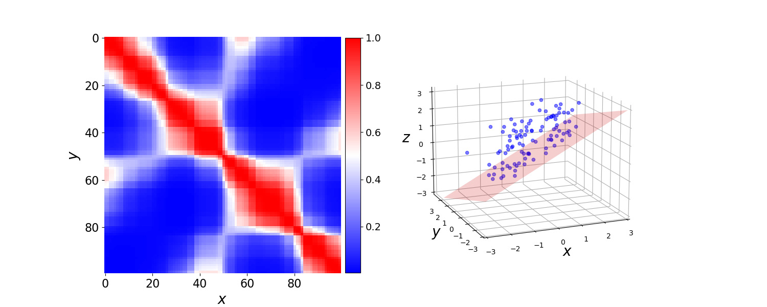
Before discussing GLS any further, let’s look at a simple example of data with heteroscedasticity and show that GLS outperforms OLS on these data. First, let’s construct a positive definite matrix with dependencies between the samples, to break the homoscedasticity assumption for OLS:

import numpy as np
from   sklearn.datasets import make_s_curve
from   sklearn.metrics.pairwise import rbf_kernel

size = 100
rng  = np.random.RandomState(seed=1)
X, t = make_s_curve(size, random_state=rng)
X    = np.delete(X, obj=1, axis=1)
X    = X / np.std(X, axis=0)
X    = X[t.argsort()]
O    = rbf_kernel(X) + 1e-6 * np.eye(size)

This constructs a covariance matrix that is definitely not just spherical errors (Figure $1$, left). Then if we assume the error terms are multivariate normal, this implies that our observations are multivariate normal, and we can construct random data (Figure $1$, right) as

from   scipy.stats import multivariate_normal

b = np.array([0.7, -0.3])
X = rng.randn(size, 2)
y = mvn(X @ b, O).rvs(random_state=rng)

Now let’s apply OLS to these data:

import statsmodels.api as sm

ols = sm.OLS(y, sm.add_constant(X)).fit()
print(ols.params[1:])   # [0.71, -0.24]
print(ols.tvalues[1:])  # [8.03, -3.01]

We can see that the inference is not great. The $t$-statistics are high, but inferred parameter values are incorrect. For example, the second parameter has a $t$-statistic over $3$ but is off from the true value by roughly $20\%$.

Figure 1. (Left) Heatmap of covariance matrix for multivariate normally distributed error terms. (Right) 100 samples drawn from $\mathbf{y} \sim \mathcal{N}(\mathbf{X}\boldsymbol{\beta}, \boldsymbol{\Omega})$. Red plane is the true hyperplane $\boldsymbol{\beta} = [0.7, -0.3]$.

Finally, let’s apply GLS rather than OLS to these data, specifying the structure of our noise terms using the sigma argument:

gls = sm.GLS(y, sm.add_constant(X), sigma=O).fit()
print(gls.params[1:])   # [0.70, -0.30]
print(gls.tvalues[1:])  # [4945.06, -2346.34]

We can see that the inference is improved. The estimated values are correct, and the $t$-stats are huge. This empirically validates the argument so far. If we know the structure of our error terms, we can still use OLS for efficient inference.

Sampling distribution

Finally, let’s derive some basic properties of GLS.

Unbiasedness. We know that the GLS estimator is unbiased, that

$\mathbb{E}\left[\hat{\boldsymbol{\beta}}_{\textsf{GLS}}\right] = \boldsymbol{\beta}. \tag{12}$

This is because Equation $10$ is unbiased, since OLS is unbiased. However, we can also follow the standard derivation for OLS unbiasedness to prove this directly:

$\begin{aligned} \mathbb{E}\left[\hat{\boldsymbol{\beta}}_{\textsf{GLS}} - \boldsymbol{\beta} \mid \mathbf{X}\right] &= \mathbb{E}[(\mathbf{X}^{\top} \boldsymbol{\Omega}^{-1} \mathbf{X})^{-1} \mathbf{X}^{\top} \boldsymbol{\Omega}^{-1} \mathbf{y} - \boldsymbol{\beta} \mid \mathbf{X}] \\ &= \mathbb{E}[(\mathbf{X}^{\top} \boldsymbol{\Omega}^{-1} \mathbf{X})^{-1} \mathbf{X}^{\top} \boldsymbol{\Omega}^{-1} (\mathbf{X} \boldsymbol{\beta} + \boldsymbol{\varepsilon}) - \boldsymbol{\beta} \mid \mathbf{X}] \\ &= \mathbb{E}[\boldsymbol{\beta} + (\mathbf{X}^{\top} \boldsymbol{\Omega}^{-1} \mathbf{X})^{-1} \mathbf{X}^{\top} \boldsymbol{\Omega}^{-1} \boldsymbol{\varepsilon} - \boldsymbol{\beta} \mid \mathbf{X}] \\ &= \mathbb{E}[(\mathbf{X}^{\top} \boldsymbol{\Omega}^{-1} \mathbf{X})^{-1} \mathbf{X}^{\top} \boldsymbol{\Omega}^{-1} \boldsymbol{\varepsilon} \mid \mathbf{X}] \\ &= (\mathbf{X}^{\top} \boldsymbol{\Omega}^{-1} \mathbf{X})^{-1} \mathbf{X}^{\top} \boldsymbol{\Omega}^{-1} \mathbb{E}[\boldsymbol{\varepsilon} \mid \mathbf{X}] \\ &= \mathbf{0}. \end{aligned} \tag{13}$

GLS estimator variance. To compute the variance of the GLS estimator, we can follow the standard derivation for the OLS variance:

$\begin{aligned} \mathbb{V}\left[\hat{\boldsymbol{\beta}}_{\textsf{GLS}} \mid \mathbf{X}\right] &= \mathbb{V} \left[\hat{\boldsymbol{\beta}}_{\textsf{GLS}} - \boldsymbol{\beta} \mid \mathbf{X} \right] \\ &= \mathbb{V} [ \overbrace{(\mathbf{X}^{\top} \boldsymbol{\Omega}^{-1} \mathbf{X})^{-1} \mathbf{X}^{\top} \boldsymbol{\Omega}^{-1}}^{\mathbf{A}} \boldsymbol{\varepsilon} \mid \mathbf{X} ] \\ &= \mathbf{A} \mathbb{V}[\boldsymbol{\varepsilon} \mid \mathbf{X}] \mathbf{A}^{\top} \\ &= \sigma^2 \mathbf{A} \boldsymbol{\Omega} \mathbf{A}^{\top} \\ &= \sigma^2 (\mathbf{X}^{\top} \boldsymbol{\Omega}^{-1} \mathbf{X})^{-1} \mathbf{X}^{\top} \boldsymbol{\Omega}^{-1} \boldsymbol{\Omega} \boldsymbol{\Omega}^{-1} \mathbf{X} (\mathbf{X}^{\top} \boldsymbol{\Omega}^{-1} \mathbf{X})^{-1} \\ &= \sigma^2 (\mathbf{X}^{\top} \boldsymbol{\Omega}^{-1} \mathbf{X})^{-1}. \end{aligned} \tag{14}$

Or we could have proved this more directly, since

$\begin{aligned} \mathbb{V}\left[\hat{\boldsymbol{\beta}}_{\textsf{OLS}} \mid \mathbf{X}_{*}\right] &= \sigma^2 (\mathbf{X}_{*}^{\top} \mathbf{X}_{*})^{-1} \\ &= \sigma^2 (\mathbf{X}^{\top} \mathbf{L}\mathbf{L}^{\top} \mathbf{X})^{-1} \\ &= \sigma^2 (\mathbf{X}^{\top} \boldsymbol{\Omega}^{-1} \mathbf{X})^{-1} \\ &= \mathbb{V}\left[\hat{\boldsymbol{\beta}}_{\textsf{GLS}} \mid \mathbf{X}\right]. \end{aligned} \tag{15}$

Unbiased GLS variance estimator. Let $\mathbf{e}$ denote the residuals, i.e.

$\mathbf{e} = \mathbf{y} - \mathbf{X} \hat{\boldsymbol{\beta}}. \tag{16}$

In OLS, an unbiased estimator of the variance, provided the OLS assumptions hold, is

$s_{\textsf{OLS}}^2 = \frac{\mathbf{e}^{\top} \mathbf{e}}{N-P}, \tag{17}$

where $P$ is the data’s dimension. Of course, we are now assuming Equation $1$, meaning the OLS assumptions do not hold. However, we can immediately derive an equivalent estimator since

$s^2 = \frac{\mathbf{e}_{*}^{\top} \mathbf{e}_{*}}{N-P} \tag{18}$

is unbiased, when $\mathbf{e}_{*} = \mathbf{y}_{*} - \mathbf{X}_{*} \hat{\boldsymbol{\beta}}$. Thus, unbiased estimator of the GLS variance is

$\begin{aligned} s_{\textsf{GLS}}^2 &= \frac{1}{N-P} (\mathbf{y}_{*} - \mathbf{X}_{*} \hat{\boldsymbol{\beta}}_{\textsf{GLS}})^{\top} (\mathbf{y}_{*} - \mathbf{X}_{*} \hat{\boldsymbol{\beta}}_{\textsf{GLS}}) \\ &= \frac{1}{N-P} (\mathbf{y} - \mathbf{X} \hat{\boldsymbol{\beta}}_{\textsf{GLS}})^{\top} \boldsymbol{\Omega}^{-1} (\mathbf{y} - \mathbf{X} \hat{\boldsymbol{\beta}}_{\textsf{GLS}}). \end{aligned} \tag{19}$

Sampling distribution. So we know the mean and variance of the sampling distribution. If we assume that the noise terms are multivariate normal,

$\boldsymbol{\varepsilon} \sim \mathcal{N}\left( \mathbf{0}, \sigma^2 \boldsymbol{\Omega} \right), \tag{20}$

then our observations are multivariate normal,

$\mathbf{y} \mid \mathbf{X} \sim \mathcal{N}\left( \mathbf{X} \boldsymbol{\beta}, \sigma^2 \boldsymbol{\Omega} \right). \tag{21}$

And the sampling distribution for the GLS estimator is also multivariate normal:

$\hat{\boldsymbol{\beta}}_{\textsf{GLS}} \mid \mathbf{X} \sim \mathcal{N}\left(\boldsymbol{\beta}, \sigma^2 (\mathbf{X}^{\top} \boldsymbol{\Omega}^{-1} \mathbf{X})^{-1} \right). \tag{22}$

Once again, this logic just follows the standard derivations for the OLS sampling distribution.

Conclusion

When our data have heteroscedasticity and when we know the structure of that heteroscedasticity, we can use generalized least squares. This is just OLS applied to the normalized data. In practice, I suspect that knowing precisely $\boldsymbol{\Omega}$ is rare, although perhaps it can be estimated from held out data. Another approach, which I will discuss in a future post, is using estimators of standard errors that are robust to heteroscedasticity.