Portfolio Theory: Why Diversification Matters

Most people with even a passing interest in financial markets have heard that diversification matters. But why? Intuitively, diversification is nice because it means you have a lower probability of losing everything at once. The idiom, “Don’t put all your eggs in one basket,” captures this intuition nicely. To my knowledge, modern portfolio theory (Markowitz, 1952), sometimes called mean–variance analysis, is the mathematical framework that first formalized this intuition. The main idea is that risk depends not just on the assets in a portfolio but the correlations among those assets, and that one does not want to simply maximize returns but to maximize risk-adjusted returns. Note that portfolio theory is not about forecasting. It does not suggest which stocks to pick. Rather, this analysis is about how to construct portfolios with desirable properties by understanding how their risks and rewards interact.

The goal of this post is to understand the basics of modern portfolio theory. As a warning to the reader, I am just starting to teach myself financial theory, and I don’t know what I don’t know here. This post is based on my notes for Prof. Andrew Lo’s 2008 course Finance Theory I at MIT.

What’s a portfolio?

We define a portfolio as a combination of $N$ assets with $N$ portfolio weights that sum to unity:

$\mathbf{w} = [ w_1, \dots, w_N ], \qquad \sum_{n=1}^N w_n = 1. \tag{1}$

Weight $w_n$ represents the proportion of the $n$th asset in the portfolio. If $M_n$ and $P_n$ are the number and price of the $n$th asset, then $w_n$ is simply the total value of the $n$th asset normalized by the value of the portfolio:

$w_n = \frac{M_n P_n}{M_1 P_1 + \dots + M_N P_N}. \tag{2}$

Weights can be negative, since we could short sell an asset (betting that an asset price will go down). Furthermore, weights could be greater than unity, meaning that we’re leveraged (trading on borrowed money). My understanding is that there are even more complicated scenarios, such as when the weights sum to zero, but I won’t discuss this here. The basic assumption, though, is that the portfolio weights summarize our investment portfolio.

Imagine for example that we had an investment account of $$10,000$ with $40$ shares of stock $A$ at $$150$ per share, $50$ shares of stock $B$ at $$20$ per share, and $25$ shares of stock $C$ at $$120$ per share. Then our portfolio with weights would be

However, the weights need not be just the proportion of a given stock or asset. For example, imagine our broker allowed us to invest on margin, meaning to buy assets while borrowing from a bank or broker, with just $$8000$ in our account to support our $$10,000$ investment. If we withdrew $$2000$ from our investment account to use for other things, then our portfolio in dollars would be unchanged, but our portfolio weights would have changed:

The weights change because the normalizer changes from $$10,000$ to $$8000$.

Defining risk and reward

Now that we have formalized portfolios, let’s define our objective. We define a desirable portfolio as a portfolio with high expected reward but low risk, where “reward” is defined as overall portfolio return and “risk” is defined as the volatility (variance or standard deviation) of that return.

These are, of course, grossly simplifying assumptions. Many investors prioritize personal or social issues over strictly higher returns. And equating risk with volatility is simplistic. In a 2014 letter to shareholders, Warren Buffett wrote:

That lesson has not customarily been taught in business schools, where volatility is almost universally used as a proxy for risk. Though this pedagogic assumption makes for easy teaching, it is dead wrong: Volatility is far from synonymous with risk.

However, this blog post is about gaining a simple mathematical foothold into the world of financial theory. Thus, I’ll make a lot of simplifying assumptions, and as I said at the beginning, I don’t know what I don’t know here. I’ll assume that returns are random variables, and that all things being equal, investors like higher expected returns with lower volatility.

Given the portfolio formulation in Equation $1$ and the goal stated above, the question becomes: how do we choose portfolio weights $\mathbf{w}$ to optimize the risk–reward characteristics of our overall portfolio? Given those weights and current stock prices $P_1, \dots, P_N$, we would then back out how much of each stock to buy, i.e. calculate $M_1, \dots, M_N$ in Equation $2$. This is the purpose of mean–variance analysis.

Diversification with uncorrelated assets

Before discussing mean–variance analysis, let’s just calculate the mean or expected return and the variance on that return for a given portfolio. Let $R_n$ denote the return on the $n$th asset in a portfolio. By definition, its mean and variance are

$\begin{aligned} \mathbb{E}[R_n] &\triangleq \mu_n, \\ \mathbb{V}[R_n] &= \mathbb{E}[(R_n - \mu_n)^2] \triangleq \sigma_n^2. \end{aligned} \tag{3}$

Now let $R_p$ denote the return on the entire portfolio; this is the quantity we’re interested in. By the linearity of expectation, we have

$\begin{aligned} R_p &\triangleq w_1 R_1 + \dots + w_N R_N, \\ &\Downarrow \\ \mathbb{E}[R_p] &= \mathbb{E}[w_1 R_1 + \dots + w_N R_N] \\ &= w_1 \mathbb{E}[R_1] + \dots + w_N \mathbb{E}[R_N] \\ &= w_1 \mu_1 + \dots + w_N \mu_N \\ &\triangleq \mu_p. \end{aligned} \tag{4}$

The first line of Equation $4$ is just an accounting identity. It’s how we would calculate the return on our portfolio given weights $\mathbf{w}$ and returns $R_1, \dots, R_N$. The variance of our portfolio’s return is

$\begin{aligned} \mathbb{V}[R_p] &= \mathbb{E}[(R_p - \mu_p)^2] \\ &= \mathbb{E}\left[ \left((w_1 R_1 + \dots + w_N R_N) - (w_1 \mu_1 + \dots + w_N \mu_N)\right)^2\right] \\ &= \mathbb{E}\left[ \left( w_1 (R_1 - \mu_1) + \dots + w_n (R_N - \mu_N) \right)^2\right] \\ &\triangleq \sigma_p^2. \end{aligned} \tag{5}$

If we have $N$ assets in our portfolio, and we square the term in the last line of Equation $5$, we get $N^2$ terms inside this expectation. We can write the variance for a single combination $R_n$ and $R_m$ as:

$\begin{aligned} \mathbb{E}[w_n w_m (R_n - \mu_n)(R_m - \mu_m)] &= w_n w_m \mathbb{E}[(R_n - \mu_n)(R_m - \mu_m)] \\ &= w_n w_m \text{Cov}[R_n, R_m] \\ &= w_n w_m \sigma_{nm} \\ &= w_n w_m \sigma_n \sigma_m \rho_{nm}, \end{aligned} \tag{6}$

where $\sigma_{nm}$ and $\rho_{nm}$ are the covariance and correlation between the $n$th and $m$th assets respectively. Equation $6$ just applies some basic definitions from probability; recall that

$\rho_{nm} = \frac{\text{Cov}[R_n, R_m]}{\sigma_n \sigma_m}. \tag{7}$

Now here’s the main point: Equation $5$ tells us that the variance of our portfolio is a function of the covariances between the assets in the portfolio. We can represent this compactly using a covariance matrix:

$\begin{bmatrix} w_1^2 \sigma_1^2 & \dots & w_1 w_N \sigma_{1N} \\ \vdots & \ddots & \vdots \\ w_N w_1 \sigma_{N1} & \dots & w_N^2 \sigma_N^2 \end{bmatrix} \quad = \quad \mathbf{w}^{\top} \begin{bmatrix} \sigma_1^2 & \dots & \sigma_{1N} \\ \vdots & \ddots & \vdots \\ \sigma_{N1} & \dots & \sigma_N^2 \end{bmatrix} \mathbf{w}. \tag{8}$

Notice, however, that there are $N$ variance terms (the diagonal of the covariance matrix in Equation $8$), while there are $N^2 - N$ covariance terms (everything else in the matrix in Equation $8$). What this means is that the correlations between assets controls our portfolio’s volatility. Positive or negative correlation between assets can increase portfolio volatility, while uncorrelated assets decrease volatility.

This starts to answer a question I had, which is, “What is diversification?” By the logic of modern portfolio theory, diversification is selecting assets that are uncorrelated, thereby reducing the variance of our portfolio’s returns. Not being diversified does not necessarily mean just owning a small number of assets. In theory, we could own a large number of assets that are all highly correlated, and the implication of Equation $5$ is that this would increase the variance in our expected returns.

Mean–variance analysis

We are now ready for the main idea of modern portfolio theory, the mean–variance analysis framework. We are going to assume that, all things being equal, investors prefer higher expected returns and lower volatility. We assume investors only care about the return on their entire portfolio, not on a single asset, i.e. they care about $R_p$, not any individual $R_n$. It’s a static analysis. Given the observed or assumed expected returns and covariances between assets, what portfolios should we prefer?

Consider Figure $1$. Here, the $x$-axis is the standard deviation of a portfolio’s return $\sigma_p$, and the $y$-axis is the expected return $\mu_p$. This is called the risk–return spectrum.

Figure 1. The risk–return spectrum: the standard deviation of an portfolio's return versus its expected value for four imaginary portfolios. Up and left is better.

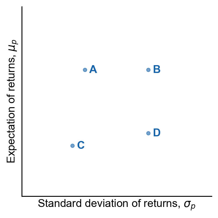
By our assumptions above, an investor should prefer portfolio $B$ over $D$, since both have the same volatility but $B$ has higher expected returns. Broadly speaking, investors want to be in the top-left corner of Figure $1$. The mean–variance analysis framework says that we want portfolio weights that push us up and left on this plot. Why? We don’t just care about expected returns but risk-adjusted returns.

How do we find the weights $\mathbf{w}$ that push a portfolio up and to the left? Imagine we have a fixed set of assets. We can estimate the expected returns, variances, and covariances however we’d like, for example, by looking at historical data. Now let $\boldsymbol{\Sigma}$ denote the covariance matrix in Equation $8$, and let $\mathbf{r}$ be an $N$-vector of expected returns, i.e. $\mathbf{r} \triangleq [\mu_1, \dots, \mu_N]$. Then the mean–variance portfolio optimization problem is:

$\begin{aligned} \min_{\mathbf{w}} &\quad \mathbf{w}^{\top} \boldsymbol{\Sigma} \mathbf{w}, \\ \text{subject to} &\quad \mathbf{w}^{\top} \mathbf{r} = K, \\ \text{and} &\quad \sum_n w_n = 1, \end{aligned} \tag{9}$

where $K$ is a user-specified hyperparameter that controls the desired expected return. In other words, we want to minimize the variance/covariance terms while ensuring our weights (1) normalize to unity and (2) give us our expected portfolio return $K$ given our estimated expected asset returns $\mathbf{r}$.

This optimization problem can be solved a number of ways, such as Lagrange multipliers, and Markowitz proposed his own approach, the critical line algorithm (Markowitz, 1955), which I won’t discuss here. Instead, I’ll discuss a simple Python solution to this problem later.

Example with two assets

Before discussing the portfolio optimization problem in Equation $9$, let’s just consider the special case of two assets, stock $A$ with weight $w_1$ and stock $B$ with weight $w_2$. This will allow us to carefully reason about what is happening. Since $w_1 + w_2 = 1$, we can easily visualize all possible portfolios by sweeping $w_1 \in [0, 1]$, calculating $w_2 \triangleq 1 - w_1$, and then computing the $(x, y)$-coordinates in the risk–reward spectrum using Equations $4$ and $5$, or for this special case:

$\begin{aligned} \mathbb{E}[R_p] &= w_1 \mu_1 + w_2 \mu_2, \\ \mathbb{V}[R_p] &= w_1^2 \sigma_1^2 + w_2 \sigma_2^2 + 2 w_1 w_2 \sigma_1 \sigma_2 \rho_{12}. \end{aligned} \tag{10}$

Now imagine that stock $A$ had an average monthly return of $2$ and a standard deviation of $10$, while stock $B$ had an average return of $1$ and a standard deviation of $6$. Suppose their correlation is $0.35$. How would a portfolio of two stocks perform? We can construct a table comparing expected portfolio return and volatility for a variety of different weights $\mathbf{w}$:

Portfolio theory does not tell us that there is necessarily a right row in this table. Which row you pick depends on where you want to be on the risk–reward spectrum. Consider the bottom row, for example, where we have shorted stock $B$. We have the highest possible expected return but also a really high standard deviation on that return.

Now let’s plot all possible portfolios with these two stocks (Figure $2$). The first thing to notice is that the risk–reward trade-off is nonlinear, a parabola induced by the functional relationship between $\mu_p$ and $\sigma_p$. Because of this shape, this parabola is sometimes referred to as the Markowitz bullet or the efficient frontier. Later, we’ll look at why it’s called “efficient”.

Figure 2. All possible portfolios for two stocks, $A$ and $B$. Holding just a single stock ($w_1 = 1$ or $w_2 = 1$), are shown as red dots. The remaining blue dots are for $w_1 \in \{0.25, 0.5, 0.75, 1.25\}$.

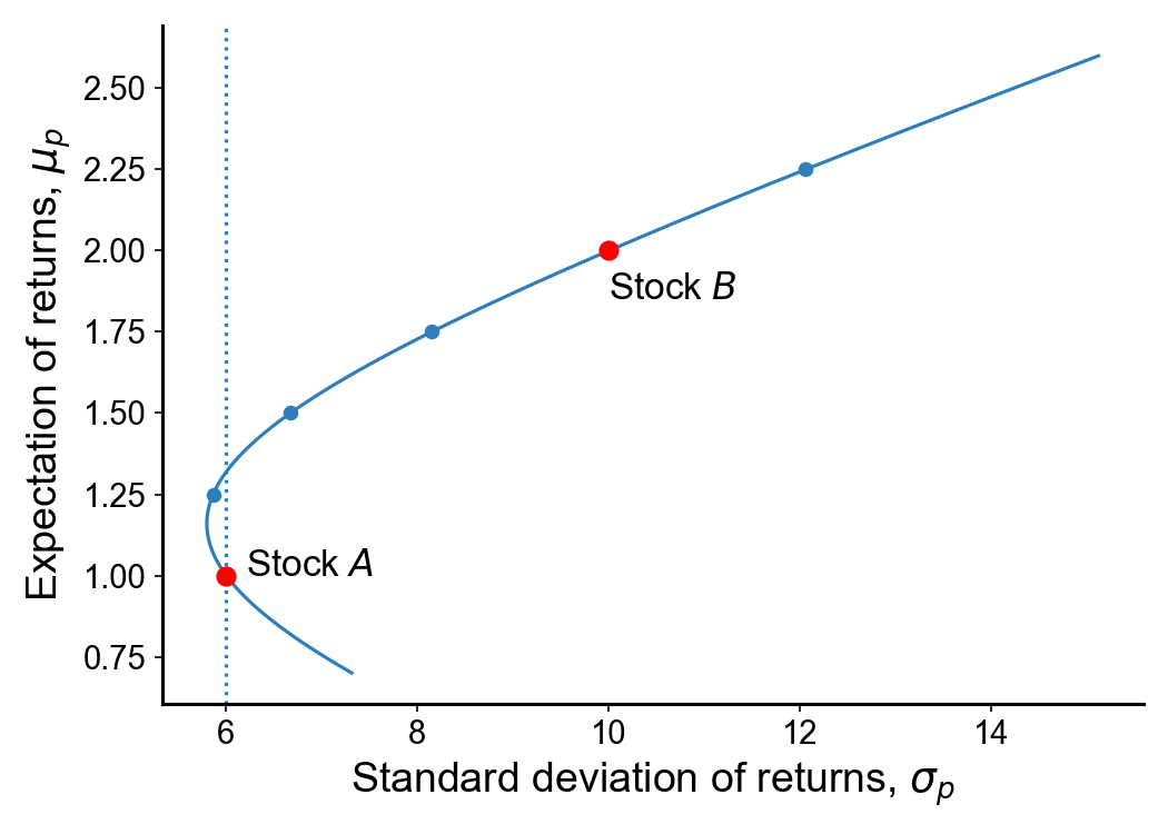
The red dots in Figure $2$ show the risk–returns of holding just stock $A$ or just stock $B$. Clearly, holding just stock $A$ is less risky than holding just $B$. However, notice that if we draw a vertical line straight up from stock $A$, we intersect the curve. This tells us that with a judicious selection of portfolio weights, we can get the same risk but with higher expected return. Everyone should prefer this point over just stock $A$. This is an example of preferring risk-adjusted expected returns, not just expected returns.

See A1 for Python code to generate Figure $2$.

Efficient frontier

Now that we have some intuition from the two-stock case, let’s discuss the more general case. In general, individual stocks do not just lie on the parabola as in Figure $2$. When $N>2$, most portfolios lie within the parabola. Any portfolio is efficient if it lies along the top half of this boundary because no other combination of assets can have smaller variance for the same expected return. This is why the Markowitz bullet is also called the efficient frontier.

We can visualize the efficient frontier in two ways. First, we can visualize many random portfolios by drawing random weights,

$\mathbf{w} \stackrel{\textsf{iid}}{\sim} \text{Dirichlet}(\boldsymbol{\alpha}), \tag{11}$

and then computing each portfolio’s $(x,y)$-coordinates of the portfolio using the equations for $\mu_p$ and $\sigma_p$. We can see the efficient frontier as the implicit parabolic edge in Figure $3$. Alternatively, we can optimize Equation $9$ to numerically approximate the weights $\mathbf{w}$ for a variety of returns (sweeping the $y$-axis) for a fixed $K$. Here, I just used SciPy’s minimize function. This produces the red line in Figure $3$. My guess is that the gaps at the edges between the sampled portfolios and the efficient frontier are due to some portfolios being highly unlikely given the Dirichlet’s distribution hyperparameters $\boldsymbol{\alpha}$.

See A2 for code to generate this figure.

Figure 3. $5000$ random portfolios, generated by drawing random weights $\mathbf{w}$ from a Dirichlet distribution with hyperparameters $\boldsymbol{\alpha} = [1,1,1,1,1]$. The red line is the efficient frontier, approximated using constrained optimization. The portfolios are colored by their Sharpe ratio.

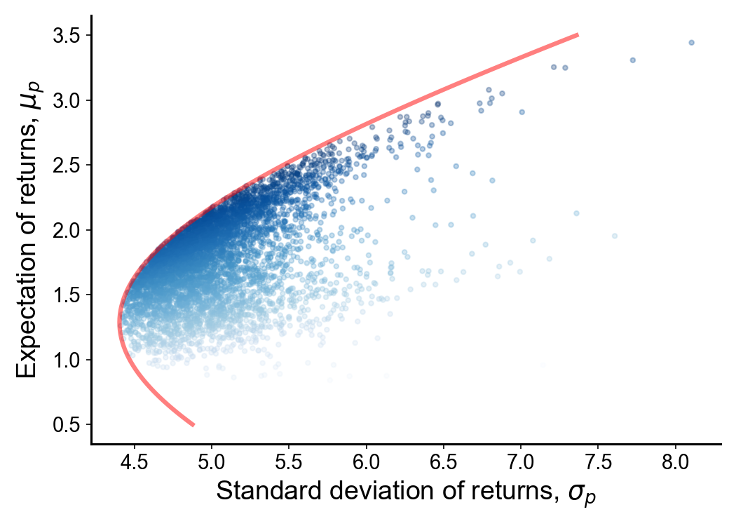
Furthermore, I’ve colored each point in Figure $3$ using the Sharpe ratio (Sharpe, 1966), defined as

$\text{Sharpe ratio} \triangleq \frac{\mu_p - r_f}{\sigma_p}, \tag{12}$

where $r_f$ is the risk-free interest rate or risk-free rate, an interest rate that is assumed to be achievable without any risk. Thus, investors often report their portfolio’s Sharpe ratio, because it quantifies the expected portfolio return, less the risk-free rate, per unit of risk. The Sharpe ratio is also related to other important ideas in portfolio theory, such as the tangent portfolio, but I won’t discuss that here.

Sometimes investors talk about alpha, which is a measure of a portfolio’s risk-adjusted performance. I haven’t seen a formal definition of alpha, but I believe it’s the numerator of the Sharpe ratio, $\mu_p - r_f$.

Limits of diversification

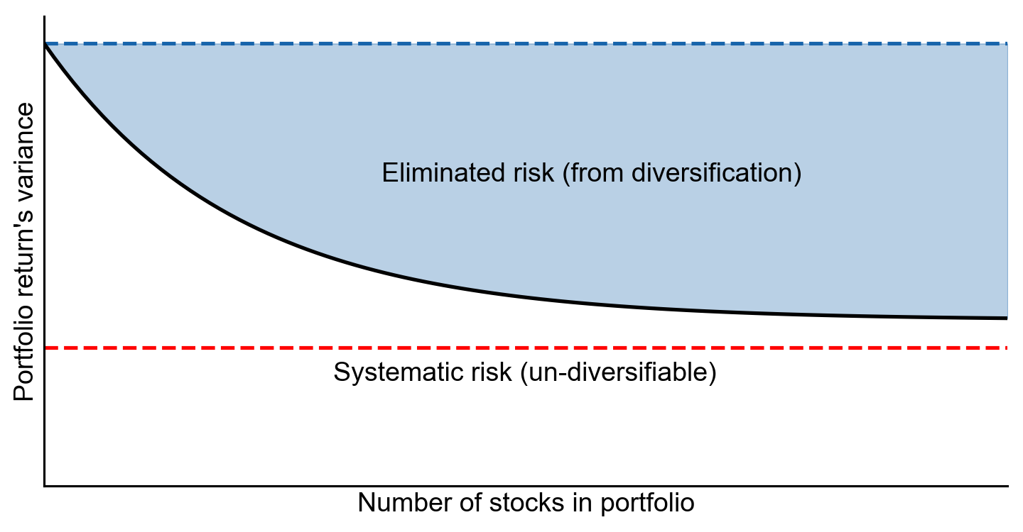
As we have seen, uncorrelated assets allow us to reduce the overall volatility in a portfolio of assets. The ups and downs are less dramatic. However, there is a diminishing effect to adding more assets to a portfolio. In the limit of an infinite number of assets, there may still exist some fundamental risk. We call this value systematic risk or market risk. It is the risk inherent to trading, and it is something all traders bear (Figure $4$).

Figure 4. A portfolio's variance decreases as the number of stocks in the portfolio (black line) increases. However, some systematic or market risk is inherent in engaging in the financial markets (red line). This risk cannot be diversified away. The difference between the total risk of a typical stock (blue line) and portfolio's risk from diversification (black line) is the risk we can eliminate through diversification (blue shaded region).

Changing correlation

As we have seen, the intuition behind, “Don’t put all your eggs in one basket,” can be expressed in finance through modern portfolio theory. Diversification means holding a portfolio of assets that are uncorrelated to reduce our risk. Of course, it is critical to remember that these correlation coefficients are not physical constants that can be estimated and then ignored. They are constantly changing, and therefore our portfolio’s volatility is constantly changing.

Again, let’s consider the special case of portfolios with just two stocks, $A$ and $B$. Now assume the correlation $\rho$ between these stocks change. What if it equals $-1$ or $0$ or $1$? Then clearly our expected return and our risk change. We can visualize the curve in Figure $2$ with different correlation coefficients $\rho$ to get a sense of how correlation effects these metrics (Figure $5$).

Figure 5. Efficient frontiers for two assets across a range of correlation coefficients $\rho$. With perfect negative correlation ($\rho = -1$), the frontier is a piecewise linear function; with no correlation ($\rho = 0$), the frontier is a Markowitz bullet; with perfect positive correlation ($\rho = 1$), the frontier is linear.

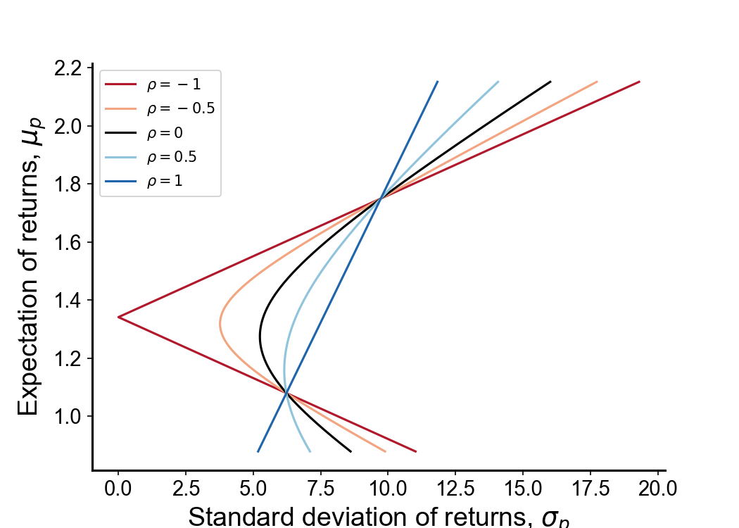
With perfect positive correlation ($\rho = 1$), the risk-reward trade-off is a straight line. The nonlinearity disappears because we effectively have the same stock, but are just holding them at different scales. With zero correlation ($\rho = 0$), we see the bump or nonlinearity as in Figure $2$. And with perfect negative correlation ($\rho = -1$), we get a piecewise linear trade-off.

One thing Figure $5$ tells us is that, if we could find two assets that are perfectly negatively correlated, then we could construct a portfolio with roughly $1.39$ return with zero risk. Of course, such perfect anti-correlation does not exist in the wild, but portfolio theory tells us how to exploit observed correlation, depending on our risk preferences.

We can estimate $\rho$ however we’d like. The obvious first thing to try in my mind would be to estimate $\rho$ from historical data.

As a warning, recall the market crash of 2008. Many investors assumed that the mortgages in their portfolios were uncorrelated or perhaps they simply ignored the correlation structure. Since the volatility in individual mortgages is quite low, this meant that a portfolio of mortgages could appear roughly risk-free. However, when the real estate market crashed, foreclosures became highly correlated, and investors’ risks changed overnight.

Conclusion

Modern portfolio theory argues that diversification reduces risk, because uncorrelated assets reduce the overall volatility of one’s portfolio. Covariance between different assets is more important than the variance of individual assets. Investors should aim for portfolios on the efficient frontier, since these portfolios have better risk-adjusted returns or bigger Sharpe ratios than portfolios inside the frontier.

Appendix

A1. Code to generate Figure $2$

import matplotlib.pyplot as plt
import numpy as np

def portfolio_perf(r, s, w, p):
    ret = np.dot(r, w)
    std = np.sqrt(np.dot(s**2, w**2) + 2 * np.prod(w) * np.prod(s) * p)
    return ret, std

r = np.array([2, 1])   # Returns.
s = np.array([10, 6])  # Standard deviations.
p = 0.35               # Correlation.

# Plot efficient frontier for w = [w1, w2].
fig, ax = plt.subplots(1, 1, figsize=(7, 5), dpi=150)
xx = np.empty(1000)
yy = np.empty(1000)
i = 0
for w1 in np.linspace(-0.3, 1.6, 1000):
    w2 = 1 - w1
    w = np.array([w1, w2])
    yy[i], xx[i] = portfolio_perf(r, s, w, p)
    i += 1
ax.plot(xx, yy, c='b', zorder=1)

# Plot portfolios at specific weight combinations.
for w1 in [0, 0.25, 0.5, 0.75, 1, 1.25]:
    w2 = 1 - w1
    w = np.array([w1, w2])
    yp, xp = portfolio_perf(r, s, w, p)
    if w1 == 0:
        ax.axvline(xp, ls=':')
        ax.text(xp+0.2, yp, 'Stock A')
    elif w1 == 1:
        ax.text(xp, yp-0.15, 'Stock B')
    c = 'r' if w1 in [0, 1] else 'b'
    size = 60 if w1 in [0, 1] else 30
    ax.scatter(xp, yp, c=c, s=size, zorder=2)

ax.set_ylabel('Expectation of returns')
ax.set_xlabel('Standard deviation of returns')
plt.show()

A2. Code to generate Figure $3$

import matplotlib.pyplot as plt
import numpy as np
from   scipy.optimize import minimize

def portfolio_perf(r, cov, w):
    ret = np.dot(r, w)
    std = np.sqrt(w.T @ cov @ w)
    return ret, std

fig, ax = plt.subplots(1, 1, figsize=(7, 5), dpi=150, sharey=True)

# Estimated expected returns and covariances.
r = np.array([2, 1, 1.3, 4, 0.5])
cov = np.array([
    [90, 22, 20, 5 , 10],
    [22, 30, 15, 20, 3 ],
    [20, 15, 40, 6 , 11],
    [5 , 20, 6 , 95, 1 ],
    [10, 3 , 11, 1 , 70]
])

# Find efficient frontier via sampling.
xx = np.empty(5000)
yy = np.empty(5000)
ss = np.empty(5000)
for i in range(5000):
    w = np.random.dirichlet([1]*5)
    yy[i], xx[i] = portfolio_perf(r, cov, w)
    ss[i] = yy[i] / xx[i]  # Sharpe ratio w/ risk-free rate == 0.
ssn = (ss - ss.min()) / (ss.max() - ss.min())
ax.scatter(xx, yy, c=ssn, cmap='Blues')

# Find efficient frontier numerically.
def efficient_portfolio(targ):
    def objective(w):
        return w.T @ cov @ w - targ * r.T @ w
    resp = minimize(objective,
                    x0=np.random.dirichlet([1]*5),
                    method='SLSQP',
                    bounds=[(-2, 2)]*5,
                    constraints=[
                        {'type': 'eq', 'fun': lambda w: 1 - w.sum()},
                        {'type': 'eq', 'fun': lambda w: np.dot(r, w) - targ}
                    ])
    return resp.x

xx = np.empty(100)
yy = np.empty(100)
# `targ` is `K` is Equation 9.
for i, targ in enumerate(np.linspace(0.5, 3.5, 100)):
    w = efficient_portfolio(targ)
    yy[i], xx[i] = portfolio_perf(r, cov, w)
ax.plot(xx, yy)

ax.set_ylabel('Expectation of returns')
ax.set_xlabel('Standard deviation of returns')
plt.show()