Standard Errors and Confidence Intervals

The standard deviation is a measure of the variation or dispersion of data, how spread out the values are. The standard error is the standard deviation of the sampling distribution. However, this does not mean that the standard error is the empirical standard deviation.¹ Since the sampling distribution of a statistic is the distribution of that statistic derived after $n$ repeated trials, the standard error is a measure of the variation in these samples. The more samples one draws, the bigger $n$ is, the smaller the standard error should be. Intuitively, the standard error answers the question: what’s the accuracy of a given statistic that we are estimating through repeated trials?

While the standard error can be estimated for other statistics, let’s focus on the mean or the standard error of the mean. Let $X = (X_1, \dots, X_n)$ denote a random sample where $X_1, \dots, X_n$ are independent and identically distributed (i.i.d.) with population variance $\sigma^2$. Because of this i.i.d. assumption, the variance of the sample mean $\bar{X} = 1/n \sum_{i=1}^n X_i$ is:

$\mathbb{V}[\bar{X}] = \mathbb{V}\left[\frac{1}{n} \sum_{i=1}^n X_i \right] = \frac{1}{n^2} \mathbb{V}\left[\sum_{i=1}^n X_i \right] = \frac{1}{n^2} (n \sigma^2) = \frac{\sigma}{\sqrt{n}} \triangleq \sigma_{\bar{x}}. \tag{1}$

If the population variance $\sigma^2$ is unknown, we can use the sample variance $\sigma_x^2$ to approximate the standard error:

$\sigma_{\bar{x}} \approx \frac{\sigma_x}{\sqrt{n}}. \tag{2}$

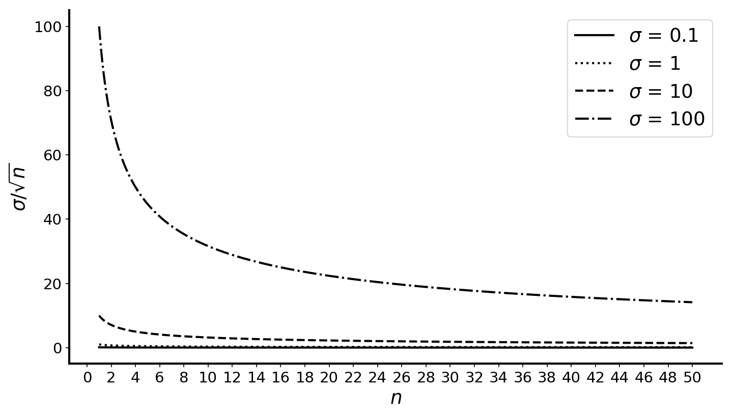
To see the effect of dividing by $n$, consider Figure $1$, which compares the standard error as a function of $n$. To reduce a given standard error by half, we need four times the number of samples:

$\frac{\sigma}{\sqrt{n}} \implies \frac{1}{2}\left( \frac{\sigma}{\sqrt{n}} \right) = \frac{\sigma}{\sqrt{4n}}. \tag{3}$

For example, when $\sigma = 100$ and $n=4$, we have a standard error of $50$. To reduce this standard error to $25$, we need $n=16$ samples.

Figure 1. The standard error $\sigma / \sqrt{n}$ as a function of $n$ and population variance.

Put differently, think about what would happen if we didn’t divide our estimate by $\sqrt{n}$. In this case, we would be just be estimating the standard deviation. This may be a nice thing to do—maybe even what we want to do—but it’s not estimating the standard deviation of the mean itself.

Confidence intervals

Standard errors are related to confidence intervals. A confidence interval specifies a range of plausible values for a statistic. A confidence interval has an associated confidence level. Ideally, we want both small ranges and higher confidence levels. Note that confidence intervals are random, since they are themselves functions of the random variable $X$.

This is a nuanced topic with a lot of common statistical misconceptions. Therefore, let’s stick to just a single simple example that illustrates this relationship. Please consult a textbook for a more thorough treatment. Imagine we want to estimate the population mean parameter $\mu$ of a random variable, which we assume is normally distributed. We can compute a standard score $Z$ as

$Z \triangleq \frac{\bar{X} - \mu}{\sigma / \sqrt{n}}. \tag{4}$

There are multiple definitions of standard score; this version tells us the difference between the sample mean $\bar{X}$ and the population mean $\mu$; this is why we normalize by the standard error rather than population variance. The units are the units of the standard error.

We can therefore compute numbers $-z$ and $z$ such that

$\mathbb{P}(-z \leq Z \leq z) = 1 - \alpha, \tag{5}$

where $1 - \alpha$ is our confidence level. If we set $\alpha = 0.05$, then we are computing the probability that the standard score is between $-z$ and $z$ with $95\%$ probability. We can compute $z$ using the cumulative distribution function $\Phi$ of the standard normal distribution, since $z$ has been normalized:

$\begin{aligned} \mathbb{P}(Z \leq z) &= \Phi(z) = 0.975, \\ &\Downarrow \\ z &= \Phi^{-1}(\Phi(z)) = \Phi^{-1}(0.975) = 1.96. \end{aligned} \tag{6}$

We’re just backing out the value $z$ given a fixed confidence level specified by $\alpha$. In other words, we decide how confident we want to be, and then estimate how big our interval must be for that desired confidence level. We can now solve for a confidence interval around the true population mean; it’s a function of our sample mean and standard score:

$\begin{aligned} 0.95 &= \mathbb{P}(-z \leq Z \leq z) \\ &= \mathbb{P}\left(-1.96 \leq \frac{\bar{X} - \mu}{\sigma / \sqrt{n}} \leq 1.96\right) \\ &= \mathbb{P} \left( \bar{X} - 1.96 \left( \frac{\sigma}{\sqrt{n}} \right) \leq \mu \leq \bar{X} + 1.96 \left( \frac{\sigma}{\sqrt{n}} \right) \right). \end{aligned} \tag{7}$

As we can see, if we compute our sample mean $\bar{X}$ and then add and subtract roughly two times the standard score, we get confidence intervals that represent the range of plausible values that the true mean parameter is in, with a confidence level of $95\%$.

Example

As an example, imagine I wanted to compare two randomized trials. A common example is a medical trial, but in machine learning research, we might want to compare two randomized algorithms, our method and a baseline. If we simply run both algorithms a few times and compare a mean metric, for example the mean accuracy, we may not be able to say anything about our model’s performance relative to the baseline. Intuitively, we may not have enough precision about the metric; and what we want to do is to increase $n$ to increase our confidence in the estimate.

Figure 2. Estimated mean and 95% confidence intervals (two standard errors) for samples from a standard normal (red) and zero-mean normal with variance $\sigma^2 = 1.1$ (blue). The bounds of the confidence intervals are shown in dashed lines.

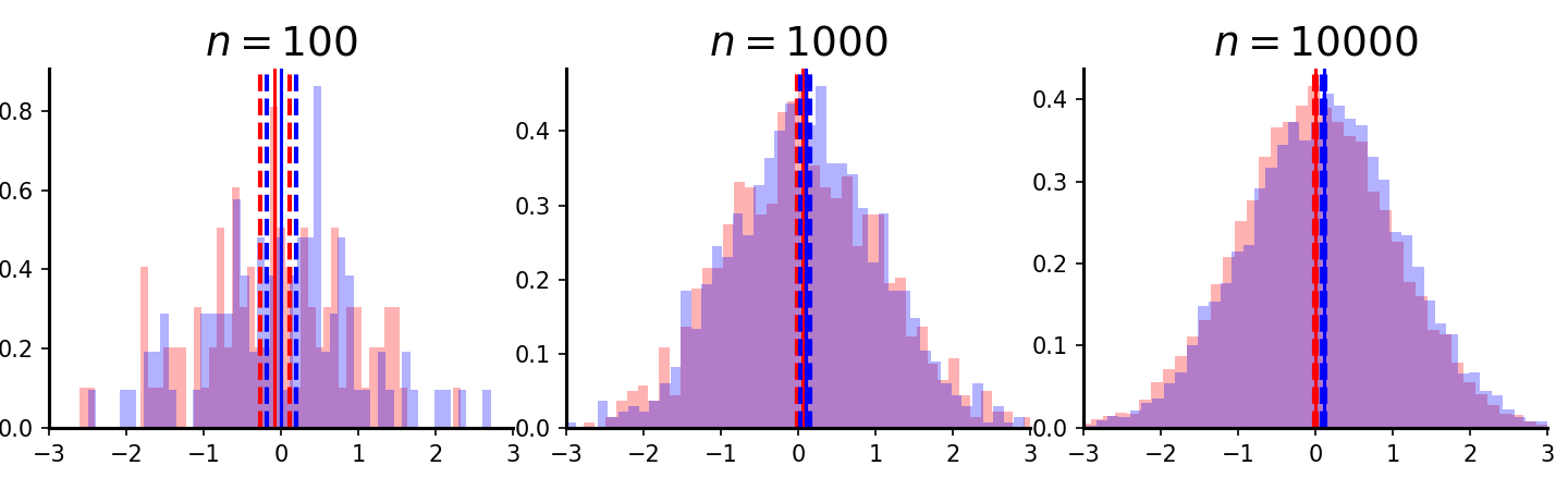
Consider Figure $2$. To generate this plot, I drew realizations $x = (x_1, \dots, x_n)$ from two normal distributions, $\mathcal{N}(0, 1)$ and $\mathcal{N}(0, 1.1)$, for increasing values of $n$. I then computed the standard score (Eq. $2$) and then plotted the $95\%$ confidence interval around the sample mean (Eq. $7$). As we can see, it is not possible to distinguish between mean estimates of the random samples, even when $n=1000$ because the confidence intervals overlap. However, when $n=10000$, we have a statistically significant result.

Conclusion

Statistical significance is a complicated topic, and I’m by no means an expert. However, just the level of background in this post demonstrates why it’s such an important topic. In my numerical experiments, I could simply increase $n$ to get confidence intervals that I desired. However, if I were running a clinical trial, I may have to fix $n$ in advance. In many machine learning papers, researchers will report the mean and standard deviation, without, I suspect, realizing that the standard deviation is simply the standard deviation of the sample (e.g. the randomized trials), not the standard deviation of the estimated mean (e.g. the average accuracy). I refer the reader again to the footnote.