Fast Computation of the Multivariate Normal PDF for Multiple Parameters
For a project, I needed to compute the log PDF of a vector for multiple pairs of mean and variance parameters. I discuss a fast Python implementation.
In a previous post, I discussed a fast and numerically stable implementation of the multivariate normal probability density function (PDF). However, for a research project, I needed to compute the log PDF of a vector for multiple sets of parameters, . This is pretty straightforward, but I want to record it in case it’s useful for others (my future self included).
Recall from my previous post that we can implement the logpdf function as
def logpdf(x, mean, cov):
    vals, vecs = np.linalg.eigh(cov)
    logdet     = np.sum(np.log(vals))
    valsinv    = 1./vals
    U          = vecs * np.sqrt(valsinv)
    dim        = len(vals)
    dev        = x - mean
    maha       = np.square(np.dot(dev, U)).sum()
    log2pi     = np.log(2 * np.pi)
    return -0.5 * (dim * log2pi + maha + logdet)
Please see that post for details. Now here is the code, with comments, for computing the same function but for multiple means and covariances:
def multiple_logpdfs(x, means, covs):
    """Compute multivariate normal log PDF over multiple sets of parameters.
    """
    # NumPy broadcasts `eigh`.
    vals, vecs = np.linalg.eigh(covs)

    # Compute the log determinants across the second axis.
    logdets    = np.sum(np.log(vals), axis=1)

    # Invert the eigenvalues.
    valsinvs   = 1./vals

    # Add a dimension to `valsinvs` so that NumPy broadcasts appropriately.
    Us         = vecs * np.sqrt(valsinvs)[:, None]
    devs       = x - means

    # Use `einsum` for matrix-vector multiplications across the first dimension.
    devUs      = np.einsum('ni,nij->nj', devs, Us)

    # Compute the Mahalanobis distance by squaring each term and summing.
    mahas      = np.sum(np.square(devUs), axis=1)

    # Compute and broadcast scalar normalizers.
    dim        = len(vals[0])
    log2pi     = np.log(2 * np.pi)
    return -0.5 * (dim * log2pi + mahas + logdets)
Above, means and covs have dimensions and respectively. Here, is the number of pairs of parameters, and is the dimension of .
We can easily verify that this code is correct:
import numpy as np
from   scipy.stats import (invwishart,
                           multivariate_normal)
from   time import perf_counter


dim   = 3
n     = 100
# Generate random data, means, and positive-definite covariance matrices.
x     = np.random.normal(size=dim)
means = np.random.random(size=(n, dim))
covs  = invwishart(df=dim, scale=np.eye(dim)).rvs(size=n)
ps1   = np.empty(n)

# Compute and time probabilities the slow way.
s = perf_counter()
for i, (m, c) in enumerate(zip(means, covs)):
    ps1[i] = multivariate_normal(m, c).logpdf(x)
t1 = perf_counter() - s

# Compute and time probabilities the fast way.
s = perf_counter()
ps2 = multiple_logpdfs(x, means, covs)
t2 = perf_counter() - s

print(t1 / t2)
assert(np.allclose(ps1, ps2))
On my computer, multiple_logpdfs is roughly two orders of magnitude faster for my (roughly ), and the slow implementation does not scale well with the number pairs of parameters (Figure ).
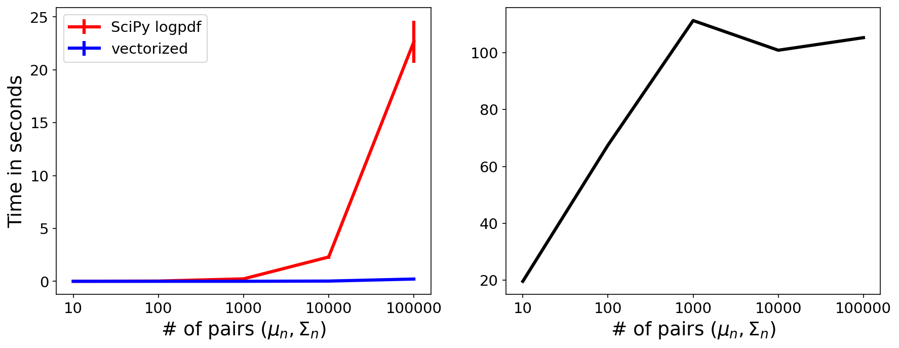
multivariate_normal.logpdf (red) and multiple_logpdfs (blue) across an increasing number of pairs of parameters . (Right) The ratio of the red curve over the blue curve. Standard deviations are computed across trials.
This speedup is not, in an absolute number of seconds, that impressive. However, my use case involves computing multiple_logpdfs inside an integral estimated using numerical quadrature, i.e. multiple_logpdfs will be called many, many times. So a speedup of two orders of magnitude is significant.
Vectorization for the input variable (27 June 2022)
Recently, someone emailed me to ask if multiple_logpdfs could be vectorized to handle x with multiple samples. Indeed, it can, and so I am adding it below. I quickly tested this numerically, but I have not used it in my own research. Please test this yourself before using it, and please email me if you find any errors.
def multiple_logpdfs_vec_input(xs, means, covs):
    """`multiple_logpdfs` assuming `xs` has shape (N samples, P features).
    """
    # NumPy broadcasts `eigh`.
    vals, vecs = np.linalg.eigh(covs)

    # Compute the log determinants across the second axis.
    logdets = np.sum(np.log(vals), axis=1)

    # Invert the eigenvalues.
    valsinvs = 1./vals

    # Add a dimension to `valsinvs` so that NumPy broadcasts appropriately.
    Us   = vecs * np.sqrt(valsinvs)[:, None]
    devs = xs[:, None, :] - means[None, :, :]

    # Use `einsum` for matrix-vector multiplications across the first dimension.
    devUs = np.einsum('jnk,nki->jni', devs, Us)

    # Compute the Mahalanobis distance by squaring each term and summing.
    mahas = np.sum(np.square(devUs), axis=2)

    # Compute and broadcast scalar normalizers.
    dim    = xs.shape[1]
    log2pi = np.log(2 * np.pi)

    out = -0.5 * (dim * log2pi + mahas + logdets[None, :])
    return out.T