Why Shouldn't I Invert That Matrix?

In a recent research meeting, I was told, “Never invert a matrix.” The person went on to explain that while we always use $\mathbf{A}^{-1}$ to denote a matrix inversion in an equation, in practice, we don’t actually invert the matrix. Instead, we solve a system of linear equations. Let me first clarify this claim. Consider solving for $\mathbf{x}$ in

$\mathbf{A} \mathbf{x} = \mathbf{b}, \tag{1}$

where $\mathbf{A}$ is an $n \times n$ matrix and $\mathbf{x}$ and $\mathbf{b}$ are $n$-vectors. One way to solve this equation is a matrix inversion $\mathbf{A}^{-1}$,

$\mathbf{x} = \mathbf{A}^{-1} \mathbf{b}. \tag{2}$

However, we could avoid computing $\mathbf{A}^{-1}$ entirely by solving the system of linear equations directly.

So why and when is one approach better than the other? John Cook has a blog post on this topic, and while it is widely referenced, it is spare in details. For example, Cook claims that “Solving the system is more numerically accurate than the performing the matrix multiplication” but provides no explanation or evidence.

The goal of this post is to expand on the why computing Eq. $2$ explicitly is often undesirable. As always, the answer lies in the details.

LU decomposition

Before comparing matrix inversion to linear system solving, we need to talk about a powerful operation that is used in both calculations: the lower–upper decomposition. Feel free to skip this section if you are familiar with this material.

The LU decomposition uses Gaussian elimination to transform a full linear system into an upper-triangular system by applying linear transformations from the left. It is similar to the QR decomposition without the constraint that the left matrix is orthogonal. Both decompositions can be used for solving linear systems and inverting matrices, but I’ll focus on the LU decomposition because, at least as I understand it, it is typically preferred in practice.

The basic idea is to transform $\mathbf{A}$ into an upper-triangular matrix $\mathbf{U}$ by repeatedly introducing zeros below the diagonal: first add zeros to the first column, then the second, and so on:

$\overbrace{\begin{bmatrix} \times & \times & \times \\ \times & \times & \times \\ \times & \times & \times \end{bmatrix}}^{\mathbf{A}} \rightarrow \overbrace{\begin{bmatrix} \times & \times & \times \\ \mathbf{0} & \times & \times \\ \mathbf{0} & \times & \times \end{bmatrix}}^{\mathbf{L}_1 \mathbf{A}} \rightarrow \overbrace{\begin{bmatrix} \times & \times & \times \\ \mathbf{0} & \times & \times \\ \mathbf{0} & \mathbf{0} & \times \end{bmatrix}}^{\mathbf{L}_2 \mathbf{L}_1 \mathbf{A}}. \tag{3}$

On the $i$-th transformation, the algorithm introduces $n-i$ zeros below the diagonal by subtracting multiples of the $(i-1)$-th row from the rows beneath it ($i+1, \dots, n$).

Let’s look at an example that borrows heavily from (Trefethen & Bau III, 1997). Consider the matrix

$\mathbf{A} = \begin{bmatrix} 2 & 1 & 1 \\ 4 & 3 & 3 \\ 8 & 7 & 9 \end{bmatrix}. \tag{4}$

First, we want to introduce zeros below the top-left $2$. Trefethen and Bau picked the numbers in $\mathbf{A}$ judiciously for convenient elimination. Namely, $A_{0,1} = 2 A_{0,0}$ and $A_{0,2} = 4 A_{0,0}$. We can represent this elimination as a lower triangular matrix $\mathbf{L}_1$ as:

$\mathbf{L}_1 \mathbf{A} = \begin{bmatrix} 1 & 0 & 0 \\ -2 & 1 & 0 \\ -4 & 0 & 1 \end{bmatrix} \begin{bmatrix} 2 & 1 & 1 \\ 4 & 3 & 3 \\ 8 & 7 & 9 \end{bmatrix} = \begin{bmatrix} 2 & 1 & 1 \\ 0 & 1 & 1 \\ 0 & 3 & 5 \end{bmatrix}. \tag{5}$

Now we just need to eliminate $3$ in $A_{2,1}$, which we can do through another linear map:

$\mathbf{L}_2 \mathbf{L}_1 \mathbf{A} = \begin{bmatrix} 1 & 0 & 0 \\ 0 & 1 & 0 \\ 0 & -3 & 1 \end{bmatrix} \begin{bmatrix} 2 & 1 & 1 \\ 0 & 1 & 1 \\ 0 & 3 & 5 \end{bmatrix} = \begin{bmatrix} 2 & 1 & 1 \\ 0 & 1 & 1 \\ 0 & 0 & 2 \end{bmatrix}. \tag{6}$

What this example highlights is that we can maintain the previously computed zeros by only operating on rows below the $i$th row.

At this point, you may note that we have computed

$\mathbf{L}_{n-1} \mathbf{L}_{n-1} \dots \mathbf{L}_1 \mathbf{A} = \mathbf{U}. \tag{7}$

Therefore, the desired lower triangular matrix requires $n-1$ inverses!

$\mathbf{L} = \mathbf{L}_1^{-1} \dots \mathbf{L}_{n-1}^{-1} \mathbf{L}_{n-1}^{-1}. \tag{8}$

As it turns out, the general formula for $\mathbf{L}_i$ is such that computing the inverse is trivial: we just negate the values below the diagonal. Please see chapter $20$ of (Trefethen & Bau III, 1997) for details.

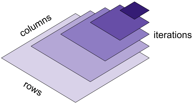
How many floating-point operations (flops) are required to compute an LU decomposition? You can find more detailed proofs elsewhere, but here’s the simple geometric intuition provided by Trefethen and Bau. For the $i$-th row in $\mathbf{A}$, we have to operate over $n - i$ columns. So for each of the $n-1$ iterations of the algorithm, we have complexity that is $(n-i) \times (n-i)$. We can visualize this as a pyramid of computation (Figure $1$).

Figure 1. Geometric intuition for the complexity of the LU decomposition. On each iteration, we perform one less operation across both the rows and columns. This results in step pyramid of computation.

Each unit of volume of this pyramid requires two flops (not discussed here), and the area of the pyramid in the limit of $n$ is $(1/3) n^3$. So the work required for LU decomposition is

$\sim \frac{2}{3} n^3 \quad \text{flops}. \tag{9}$

Solving a linear system

Now let’s talk about using the LU decomposition to solve a linear system. Let the notation $\mathbf{A} \setminus \mathbf{b}$ denote the vector $\mathbf{x}$ that solves $\mathbf{A x} = \mathbf{b}$. How do we compute $\mathbf{x}$ without using a matrix inverse? A standard method is to use the LU decomposition of $\mathbf{A}$ and then solve two easy systems of equations:

$\begin{aligned} \mathbf{Ax} &= \mathbf{b}, \\ \mathbf{LUx} &= \mathbf{b}, && \text{(LU decomposition)} \\ \mathbf{L} \setminus \mathbf{b} &= \mathbf{y}, && \text{(forward substitution)} \\ \mathbf{U} \setminus \mathbf{y} &= \mathbf{x}, && \text{(backward substitution)} \\ &\Downarrow \\ \mathbf{LUx} &= \mathbf{Ly} = \mathbf{b}. \end{aligned} \tag{10}$

Why is it easy to solve for $\mathbf{y}$ and $\mathbf{x}$ w.r.t. $\mathbf{L}$ and $\mathbf{U}$ respectively? Because these are lower- and upper-triangular matrices respectively. For example, consider solving for $\mathbf{y}$ above:

$\begin{bmatrix} 1 \\ \ell_{2,1} & 1 \\ \vdots & \dots & \ddots \\ \ell_{n-1,1} & \dots & \dots & 1 \\ \ell_{n,1} & \dots & \dots & \ell_{n,n-1} & 1 \end{bmatrix} \begin{bmatrix} y_1 \\ y_2 \\ \vdots \\ y_{n-1} \\ y_n \end{bmatrix} = \begin{bmatrix} b_1 \\ b_2 \\ \vdots \\ b_{n-1} \\ b_n \end{bmatrix} \tag{11}$

For each value $y_i$, we have

$y_i = b_i - \ell_{i,1} y_1 - \dots - \ell_{i,i-1} y_{i-1}. \tag{12}$

Solving for $\mathbf{y}$ in this way is called forward substitution because we compute $y_1$ and then forward substitute the value into the next row and so on. We can then run backward substitution on an upper-triangular matrix—so starting at the bottom row and moving up—to solve for $\mathbf{x}$.

What’s the cost of this computation? Forward substitution requires $i-1$ multiplications and subtractions at each step or

$2 \sum_{i=1}^n (i-1) = \big( 2 \sum_{i=1}^n i \big) - n = n^2 - n. \tag{13}$

The cost of backward substitution is slightly larger because the diagonal elements are not one. Therefore, there are $n$ additional divisions or $n^2$ flops. Therefore the total complexity of solving a linear system of equations using the LU decomposition is

$\sim \frac{2}{3} n^3 + 2 n^2 \quad \text{flops}. \tag{14}$

Inverting a matrix

Now let’s consider inverting a matrix. Now that we understand the LU decomposition, matrix inversion is easy. We want to compute $\mathbf{A}^{-1}$ in

$\mathbf{AA}^{-1} = \mathbf{I} = \left[\begin{array}{c|c|c|c} \textbf{e}_1 & \textbf{e}_2 & \vdots & \textbf{e}_n \\\\ \end{array}\right] \tag{15}$

Once we have the LU decomposition, we can simply solve for each column of $\mathbf{I}$:

$\mathbf{LUx}_i = \mathbf{e}_i. \tag{16}$

The simplest algorithm would be to perform this operation $n$ times. Since the LU decomposition requires $(2/3) n^3$ flops and solving for each $\mathbf{x}_i$ requires $2n^2$ flops, we see that that matrix inversion requires

$\sim \frac{8}{3} n^3 \quad \text{flops.} \tag{17}$

That said, matrix inversion is a complicated topic, and there are faster algorithms. But the basic idea is that the inversion itself is not faster than the LU decomposition, which effectively solves for $\mathbf{x}$.

Finally, solving for $\mathbf{A}^{-1}$ is not the same thing as computing $\mathbf{x}$. To compute $\mathbf{x}$, we have to perform a matrix multiplication, $\mathbf{A}^{-1} \mathbf{b}$, which is

$\sim 2 n^3 \quad \text{flops.} \tag{18}$

As we can see inverting a matrix to solve $\mathbf{Ax} = \mathbf{b}$ is roughly three times as expensive as directly solving for $\mathbf{x}$. This alone is justification for the claim that, unless you have good reasons, it is better to directly solve for $\mathbf{x}$.

Numerical errors and conditioning

As we’ll see, solving a linear system using a matrix inverse can also be less accurate. However, before discussing this, let’s review several concepts related to numerical methods. Consider the function

$y = f(x), \tag{19}$

and imagine we can only approximate its output, denoted $\hat{y}$. The forward error is the error between the true and approximated outputs, $\left| \hat{y} - y \right|$. The backward error measures the sensitivity to the problem. We want the smallest $\Delta x$ such that

$\hat{y} = f(x + \Delta x). \tag{20}$

This quantifies: for what input data have we actually solved the problem? If $\Delta x$ is very large, then our approximation $\hat{y}$ isn’t even based on a value close to the true input $x$. So $\left| \Delta x \right|$ is called the backward error.

For example, imagine we approximate $\sqrt{2}$ with $1.4$. The forward error is the absolute difference between $1.4$ and $\sqrt{2}$. Since $\sqrt{1.96} = 1.4$, the backward error is the absolute difference between $2$ and $1.96$.

Finally, we say that the problem $y = f(x)$ is well-conditioned if a small change in $x$ leads to a small change $y$ and ill-conditioned otherwise. This is often quantified with a condition number. In numerical linear algebra, the condition number of a matrix, denoted by $\kappa(\mathbf{A})$, is

$\kappa(\mathbf{A}) = \lVert \mathbf{A} \rVert \lVert \mathbf{A}^{-1} \rVert. \tag{21}$

If $\lVert \cdot \rVert$ is the matrix $2$-norm, then Eq. $21$ is just the ratio of largest to smallest singular values,

$\kappa(\mathbf{A}) = \frac{\lambda_1}{\lambda_n}. \tag{21}$

See this StackExchange answer for a proof. In other words, an ill-conditioned matrix is one with a large spread in its singular values. Intuitively, this is not surprising, since matrices with sharp decays in their singular values are associated with many other instabilities, such as in control systems.

Accuracy

Let’s return to the main thread. A second problem with matrix inversion is that it can be less accurate. Let $\mathbf{x}_{\texttt{LU}}$ denote the vector solved for directly by the LU decomposition, and let $\mathbf{x}_{\texttt{inv}}$ denote the vector solved by $\text{inv}(\mathbf{A}) \times \mathbf{b}$, where $\text{inv}(\mathbf{A})$ is computed using the LU decomposition as discussed above. Now imagine that we computed the matrix inverse exactly, meaning we have no rounding errors in the computation $\text{inv}(\mathbf{A})$. Then the best residual bound on the backward error, taken from section $14.1$ of (Higham, 2002), is:

$\left| \mathbf{b} - \mathbf{A} \mathbf{x}_{\texttt{inv}} \right| \leq \textcolor{#8e7cc3}{\gamma_n \left| \mathbf{A} \right|} \left| \mathbf{A}^{-1} \right| \left| \mathbf{b} \right|, \tag{22}$

where $\gamma_n$ is a small constant factor accounting for things like machine precision. For $\mathbf{x}_{\texttt{LU}}$, this bound is

$\left| \mathbf{b} - \mathbf{A} \mathbf{x}_{\texttt{LU}} \right| \leq \textcolor{#8e7cc3}{\gamma_n \left| \mathbf{L} \right| \left| \mathbf{U} \right|} \left| \mathbf{x}_{\texttt{LU}} \right|. \tag{23}$

If we assume the LU decomposition of $\mathbf{A}$ is relatively good—something Higham says is “usually true”—then the terms in purple in Eq. $22$ and $23$ are roughly equal, and the terms that dominate the bound for each method are $\left| \mathbf{x}_{\texttt{LU}} \right|$ and $\left| \mathbf{A}^{-1} \right| \left| \mathbf{b} \right|$. Thus, the matrix inversion approach can have signficantly worse backward error than directly solving for $\mathbf{x}$ if the matrix $\mathbf{A}$ is ill-conditioned.

That said, the forward error between matrix inversion and direct solving can be much closer than expected for well-conditioned problems, a point argued by (Druinsky & Toledo, 2012). Thus, in practice, if you care only about the forward error, the folk wisdom that you should never invert a matrix may stress the point too much. I don’t discuss the bounds on forward errors here, but see this StackExchange post for details.

As I see it, the upshot is still the same: solving a system of linear equations by performing a matrix inversion is typically less accurate than solving the system directly.

Numerical experiments

I ran a couple simple numerical experiments to verify the results discussed above.

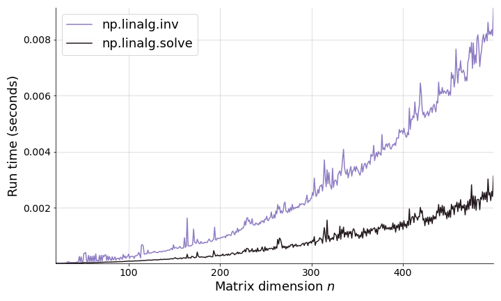
First, let’s explore whether in practice, solving for $\mathbf{x}$ directly is faster than using a matrix inversion. For increasing $n$, I ran the following experiment: generate a matrix $\mathbf{A}$ and vector $\mathbf{b}$. Then solve for $\mathbf{x}$ using np.linalg.solve(A, b) and np.linalg.inv(A) @ b. I ran each experiment $10$ times and recorded the mean run time (Figure $2$). As expected, solving for $\mathbf{x}$ directly is faster. While the absolute difference in seconds is trivial here, it is easy to imagine this mattering more in large-scale data processing tasks.

Figure 2. Mean run time to compute $\mathbf{x}$ in $\mathbf{Ax} = \mathbf{b}$ over $10$ trials and increasing matrix dimension $n$ using both a matrix inversion and a linear solver.

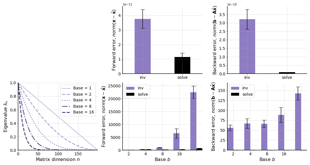
Next, let’s explore the forward and backward error for well- and ill-conditioned problems. I generated two matrices $\mathbf{A}_w$ and $\mathbf{A}_i$ in the following way:

x = np.random.normal(n)

# Well-conditioned A and resulting b.
Aw = np.random.normal(size=(n, n))
bw = Aw @ x

# Ill-conditioned A and resulting b.
lambs = np.power(np.linspace(0, 1, n), b)
inds  = np.argsort(lambs)[::-1]
lambs = lambs[inds]

Q  = ortho_group.rvs(dim=n)
Ai = Q @ np.diag(lambs) @ Q.T
bi = Ai @ x

In words, the well-conditioned matrix is just a full-rank matrix with each element drawn from $\mathcal{N}(0, 1)$. For the ill-conditioned matrix, I generated a matrix with sharply decaying singular values. The decay rate is controlled by an exponent base b. As we can see (Figure $3$), both the forward and backward errors are relatively small and close to each other when the matrix is well-conditioned. However, when the matrix is ill-conditioned, the forward and backward errors increase, loosely as a function of the decay rate for the singular values.

Figure 3. (Top row) Forward and backward errors for $\mathbf{x}_{\texttt{inv}}$ and $\mathbf{x}_{\texttt{LU}}$ on a well-conditioned matrix. (Bottom row) Forward and backward errors for $\mathbf{x}_{\texttt{inv}}$ and $\mathbf{x}_{\texttt{LU}}$ on ill-conditioned matrices. The singular values decay w.r.t. to various exponent bases (bottom left).

Summary

When solving for $\mathbf{x}$ in $\mathbf{Ax} = \mathbf{b}$, it is always faster and often more accurate to directly solve the system of linear equations, rather than inverting $\mathbf{A}$ and doing a left multiplication with $\mathbf{b}$. This is a big topic, and I’m sure I’ve missed many nuances, but I think the main point stands: as a rule, one should be wary of inverting matrices.