Gaussian Process Dynamical Models

A Gaussian process dynamical model (GPDM) (Wang et al., 2006) can be viewed as a Gaussian process latent variable model (GPLVM) with the latent variable evolving according to its own Gaussian process. Put more simply, imagine a latent variable evolves according to some smooth, nonlinear dynamics, and that the mapping from latent- to observation-space is also a smooth, nonlinear map. For example, imagine a mouse is moving in a maze, but we only record the firing rates of its hippocampal place cells. The latent variable is the mouse position, which we know is a relatively smooth trajectory in 3D space, and the observations, neuron firing rates, are a nonlinear function of this latent variable. Can we infer the position of the mouse given just its firing rates? This is the type of question the GPDM attempts to answer. The goal of this post is to work through this model in detail.

Gaussian process dynamics

Let $\mathbf{Y} = [\mathbf{y}_1 \dots \mathbf{y}_T]^{\top}$ be $T$ observations, each $J$-dimensional, and indexed by discrete-time index $t$, and let $\mathbf{X} = [\mathbf{x}_1 \dots \mathbf{x}_T]^{\top}$ be $D$-dimensional latent variables. Now consider the following Markov dynamics:

$\begin{aligned} \mathbf{x}_t &= f(\mathbf{x}_{t-1}; \mathbf{A}) + \mathbf{n}_{x,t}, \\ \mathbf{y}_t &= g(\mathbf{x}_{t}; \mathbf{B}) + \mathbf{n}_{y,t}. \end{aligned} \tag{1}$

In Eq. $1$, $f$ and $g$ are mappings with parameters $\mathbf{A}$ and $\mathbf{B}$ respectively, and $\mathbf{n}_{x,t}$ and $\mathbf{n}_{y,t}$ are zero-mean Gaussian noise. The latent dynamics are Markov because the latent variable at time $t$, $\mathbf{x}_t$, only depends on the previous latent variable $\mathbf{x}_{t-1}$ and the dynamics defined by $f$. Each observation $\mathbf{y}_t$ depends on its latent variable $\mathbf{x}_t$ through the function $g$. For example, in a linear dynamical system, $f$ and $g$ are linear functions:

$\begin{aligned} \mathbf{x}_t &= \mathbf{A} \mathbf{x}_{t-1} + \mathbf{n}_{x,t}, \\ \mathbf{y}_t &= \mathbf{B} \mathbf{x}_{t} + \mathbf{n}_{y,t}. \end{aligned} \tag{2}$

In the original GPDM paper, the authors propose a particular nonlinear case in which $f$ and $g$ are linear combinations of basis functions:

$\begin{aligned} f(\mathbf{x}; \mathbf{A}) &= \sum_{k=1}^{K} \mathbf{a}_k \phi_k(\mathbf{x}), \\ g(\mathbf{x}; \mathbf{B}) &= \sum_{m=1}^{M} \mathbf{b}_m \psi_m(\mathbf{x}), \end{aligned} \tag{3}$

for weights $\mathbf{A} = [\mathbf{a}_1 \dots \mathbf{a}_K]^{\top}$ and $\mathbf{B} = [\mathbf{b}_1 \dots \mathbf{b}_M]^{\top}$. To be clear, this is just a matrix-vector multiplication. We can rewrite Eq. $3$ as

$\begin{aligned} f(\mathbf{x}; \mathbf{A}) &= \underbrace{ \left[\begin{array}{c|c|c} \mathbf{a}_1 & \dots & \mathbf{a}_K \end{array}\right] }_{\mathbf{A}} \underbrace{ \begin{bmatrix} \phi_1(\mathbf{x}) \\ \vdots \\ \phi_K(\mathbf{x}) \end{bmatrix} }_{\boldsymbol{\phi}(\mathbf{x})}, \\ g(\mathbf{x}; \mathbf{B}) &= \underbrace{ \left[\begin{array}{c|c|c} \mathbf{b}_1 & \dots & \mathbf{b}_M \end{array}\right] }_{\mathbf{B}} \underbrace{ \begin{bmatrix} \psi_1(\mathbf{x}) \\ \vdots \\ \psi_M(\mathbf{x}) \end{bmatrix} }_{\boldsymbol{\psi}(\mathbf{x})}, \end{aligned} \tag{4}$

where $\mathbf{A}$ and $\mathbf{B}$ are $D \times K$ and $J \times M$ matrices respectively and where $\boldsymbol{\phi}(\mathbf{x}) = [\phi_1(\mathbf{x}) \dots \phi_K(\mathbf{x})]^{\top}$ and $\boldsymbol{\psi}(\mathbf{x}) = [\psi_1(\mathbf{x}) \dots \psi_M(\mathbf{x})]^{\top}$, so $K$- and $M$-vectors respectively.

It may not be obvious why this is a clever idea, but if we place Gaussian priors on the rows of $\mathbf{A}$ and $\mathbf{B}$, we can integrate them out. In both cases, the derivations are the same, minus a few details, as the derivation for a GPLVM. We will be left with multivariate Gaussian distributions whose covariance matrices are Gram matrices where each cell value is a dot product between the basis functions, e.g.

$\mathbf{K}_{ij} = \phi_i(\mathbf{x})^{\top} \phi_j(\mathbf{x}). \tag{5}$

Thus, an appropriate choice of basis function implies Gaussian-process dynamics for this model. This is a common theme in Bayesian inference: placing a prior on weights induces a prior on functions.

Now let’s walk through this integration process in detail.

Integrating out the weights

First, let’s integrate out $\mathbf{B}$. Wang’s modeling assumption is that each row of $\mathbf{B}$, each $\mathbf{b}_j$, has a isotropic Gaussian prior, meaning

$p(\mathbf{B}) = \prod_{j=1}^{J} \mathcal{N}_M( \mathbf{b}_j \mid \mathbf{0}, w_j^{-2} \mathbf{I}), \tag{6}$

for some variance $w_j^{-2}$. Now let’s rewrite the model in terms in terms of the features (columns) of $\mathbf{Y}$:

$\mathbf{y}_j = \boldsymbol{\Psi} \mathbf{b}_j + \mathbf{n}_{y,j}, \tag{7}$

where $\boldsymbol{\Psi} = [\boldsymbol{\psi}(\mathbf{x}_1) \dots \boldsymbol{\psi}(\mathbf{x}_T)]^{\top}$, or a $T \times M$ matrix. This implies that the distribution on $\mathbf{y}_j$, conditioned on $\mathbf{b}_j$, is a $T$-variate normal,

$\mathbf{y}_j \mid \mathbf{X}, \mathbf{b}_j \sim \mathcal{N}_T(\mathbf{y}_j \mid \boldsymbol{\Psi} \mathbf{b}_j, w_j^{-2} \sigma_Y^2 \mathbf{I}). \tag{8}$

Note that the variance of $\mathbf{n}_{y,j}$ is $w_j^{-2} \sigma_Y^2$. Wang never writes this out explicitly, but he doesn’t write out many terms explicitly, and this assumption makes the derivation work. Since both $p(\mathbf{b}_j)$ and $p(\mathbf{y}_j \mid \mathbf{b}_j)$ are independently Gaussian, we can marginalize out $\mathbf{b}_j$ to get:

$p(\mathbf{y}_j \mid \mathbf{X}) = \mathcal{N}_T(\mathbf{y}_j \mid \mathbf{0}, \boldsymbol{\Psi} w_j^{-2} \boldsymbol{\Psi}^{\top} + w_j^{-2} \sigma_Y^2 \mathbf{I}). \tag{9}$

See Sec. $2.3.3$ in (Bishop, 2006) if this marginalization does not make sense. We can rewrite the covariance matrix in Eq. $9$ as

$\boldsymbol{\Psi} w_j^{-2} \boldsymbol{\Psi}^{\top} + w_j^{-2} \sigma_Y^2 \mathbf{I} = w_j^2 (\boldsymbol{\Psi} \boldsymbol{\Psi}^{\top} + \sigma_Y^2 \mathbf{I}) = w_j^2 \mathbf{K}_Y, \tag{10}$

where we’ve defined $\mathbf{K}_Y = \boldsymbol{\Psi} \boldsymbol{\Psi}^{\top} + \sigma_Y^2 \mathbf{I}$. Therefore, the joint density over all $J$ features is

$\begin{aligned} p(\mathbf{Y} \mid \mathbf{X}) &= \prod_{j=1}^{J} p(\mathbf{y}_j \mid \mathbf{X}) \\ &= \prod_{j=1}^{J} \frac{1}{\sqrt{(2\pi)^T |w_j^{-2} \mathbf{K}_Y|}} \exp\Big\{ -\frac{1}{2} \mathbf{y}_j^{\top} w_j^{-2} \mathbf{K}_Y^{-1} \mathbf{y}_j \Big\} \\ &= \frac{(w_j)^{TJ}}{\sqrt{(2\pi)^{TJ} |\mathbf{K}_Y|^J}} \exp\Big\{-\frac{1}{2} \sum_{j=1}^{J} \mathbf{y}_j^{\top} w_j^{-2} \mathbf{K}_Y^{-1} \mathbf{y}_j \Big\} \\ &= \frac{(w_j)^{TJ}}{\sqrt{(2\pi)^{TJ} |\mathbf{K}_Y|^J}} \exp\Big\{-\frac{1}{2} \text{tr} \Big( \sum_{j=1}^{J} \mathbf{K}_Y^{-1} \mathbf{y}_j \mathbf{y}_j^{\top} w_j^{-2} \Big) \Big\} \\ &= \frac{|\mathbf{W}|^{T}}{\sqrt{(2\pi)^{TJ} |\mathbf{K}_Y|^J}} \exp\Big\{-\frac{1}{2} \text{tr} \Big( \mathbf{K}_Y^{-1} \mathbf{Y} \mathbf{W}^2 \mathbf{Y}^{\top} \Big) \Big\}, \end{aligned} \tag{11}$

where $\mathbf{W} = \text{diag}([w_1 \dots w_J])$. We have used a trace trick, the fact that the sum of outer products is a matrix multiplication, and some properties of the determinant. Thus, we have rederived Wang’s Eq. $5$.

Now let’s integrate out $\mathbf{A}$. The assumption is that rows of $\mathbf{A}$ are i.i.d. Gaussian,

$p(\mathbf{A}) = \prod_{d=1}^D \mathcal{N}_K(\mathbf{a}_d \mid \mathbf{0}, \mathbf{I}). \tag{12}$

We can rewrite Eq. $4$ in terms of the columns of $\mathbf{X}$ and the rows of $\mathbf{A}$:

$\begin{aligned} \mathbf{x}_d^{(2:T)} &= \boldsymbol{\Phi}^{1:(T-1)} \mathbf{a}_d + \mathbf{n}_{x,d}, \\ &\Downarrow \\ \mathbf{x}_d^{(2:T)} \mid \mathbf{X}, \mathbf{a}_d &\sim \mathcal{N}_{T-1}(\mathbf{x}_d^{(2:T)} \mid \boldsymbol{\Phi}^{1:(T-1)} \mathbf{a}_d, \sigma^2_X \mathbf{I}), \end{aligned} \tag{13}$

where $\mathbf{x}_d^{(2:T)}$ denotes the $d$-th column of $\mathbf{X}$ after removing the first row of $\mathbf{X}$, i.e. $\mathbf{x}_d^{(2:T)} = [x_d^{(2)} \dots x_d^{(T)}]^{\top}$, and where $\boldsymbol{\Phi}^{1:(T-1)} = [\boldsymbol{\phi}(\mathbf{x}_1) \dots \boldsymbol{\phi}(\mathbf{x}_{T-1})]^{\top}$. To be clear, the superscripts denote components in a vector. $\sigma_X^2$ is the variance of $\mathbf{n}_{x,d}$. This funky indexing is just the result of the Markov assumption, that $\mathbf{x}_{t}$ depends on $\mathbf{x}_{t-1}$. Since this superscript notation is quite unwieldly, we’ll drop it in favor of just specifying matrix shapes as needed. Again, we can marginalize out $\mathbf{A}$ since both $p(\mathbf{x}_d \mid \mathbf{a}_d)$ and $p(\mathbf{a}_d)$ are Gaussian:

$p(\mathbf{x}_d) = \mathcal{N}_{T-1}(\mathbf{x}_d \mid \mathbf{0}, \underbrace{\boldsymbol{\Phi}\boldsymbol{\Phi}^{\top} + \sigma_X^2 \mathbf{I}}_{\mathbf{K}_X}). \tag{14}$

Again, see Sec. $2.3.3$ in (Bishop, 2006) if this marginalization does not make sense. Thus, we can marginalize out $\mathbf{A}$ from the model entirely:

$\begin{aligned} p(\mathbf{X}) &= \int p(\mathbf{X} \mid \mathbf{A}) p(\mathbf{A}) \text{d}\mathbf{A} \\ &= \int p(\mathbf{x}_1) \prod_{d=1}^D p(\mathbf{x}_d \mid \mathbf{A}) p(\mathbf{A}) \text{d}\mathbf{A} \\ &= p(\mathbf{x}_1) \prod_{d=1}^D \frac{1}{\sqrt{(2\pi)^{(T-1)}|\mathbf{K}_X|}} \exp\Big\{-\frac{1}{2} \mathbf{x}_d^{\top} \mathbf{K}_X^{-1} \mathbf{x}_d \Big\} \\ &= p(\mathbf{x}_1) \frac{1}{\sqrt{(2\pi)^{D(T-1)}|\mathbf{K}_X|^D}} \exp\Big\{-\frac{1}{2} \sum_{d=1}^{D} \mathbf{x}_d^{\top} \mathbf{K}_X^{-1} \mathbf{x}_d \Big\} \\ &= p(\mathbf{x}_1) \frac{1}{\sqrt{(2\pi)^{D(T-1)}|\mathbf{K}_X|^D}} \exp\Big\{-\frac{1}{2} \text{tr} \big( \mathbf{K}_X^{-1} \bar{\mathbf{X}} \bar{\mathbf{X}}^{\top} \big) \Big\}, \end{aligned} \tag{15}$

where $\bar{\mathbf{X}} = \mathbf{X}^{(2:T)}$.

That’s it. We have derived the GPDM. As with the derivation for a GPLVM, it may not be immediately obvious where the Gaussian processes are, but notice that both $p(\mathbf{Y} \mid \mathbf{X})$ and $p(\mathbf{X})$ are both multivariate Gaussian with covariance matrices that are functions of Gram matrices, $\mathbf{K}_Y$ and $\mathbf{K}_X$. The other matrices in the last lines of Eq. $11$ and $15$ are the column-specific variances, $\mathbf{W}$, or the result of the i.i.d. assumption for the observations and latent variables, $\mathbf{Y}$ and $\bar{\mathbf{X}}$. Thus, this model implies a Gaussian process prior on both the dynamics and latent-to-observation maps if we define $\mathbf{K}_Y$ and $\mathbf{K}_X$ using positive definite kernel functions.

Inference

We want to infer the posterior $p(\mathbf{X} \mid \mathbf{Y})$ where

$p(\mathbf{X} \mid \mathbf{Y}) \propto p(\mathbf{Y} \mid \mathbf{X}) p(\mathbf{X}). \tag{16}$

Therefore, the log posterior in Eq. $16$ decomposes into the sum of the logs of Eq. $11$ and $15$:

$\begin{aligned} &\mathcal{L}(\mathbf{X}) \\ &= \log p(\mathbf{Y} \mid \mathbf{X}) + \log p(\mathbf{X}) \\ &= T \log |\mathbf{W}| - \cancel{\frac{TJ}{2} \log(2\pi)} - \frac{J}{2} \log |\mathbf{K}_Y| - \frac{1}{2} \text{tr}(\mathbf{K}_Y^{-1} \mathbf{Y} \mathbf{W} \mathbf{Y}^{\top}) \\&+ \cancel{\frac{D(T-1)}{2} \log(2\pi)} - \frac{D}{2} \log |\mathbf{K}_X| - \frac{1}{2} \text{tr}(\mathbf{K}_X^{-1} \bar{\mathbf{X}} \bar{\mathbf{X}}^{\top}) + \cancel{\log p(\mathbf{x}_1)} \\ &= T \log |\mathbf{W}| - \frac{J}{2} \log |\mathbf{K}_Y| - \frac{1}{2} \text{tr}(\mathbf{K}_Y^{-1} \mathbf{Y} \mathbf{W} \mathbf{Y}^{\top}) - \frac{D}{2} \log |\mathbf{K}_X| - \frac{1}{2} \text{tr}(\mathbf{K}_X^{-1} \bar{\mathbf{X}} \bar{\mathbf{X}}^{\top}). \end{aligned} \tag{17}$

We can cancel constant terms. If we optimize the latent variable $\mathbf{X}$ with respect to this log posterior, Eq. $17$, then we will infer a latent variable that adheres to our modeling assumptions in Eq. $3$. However, Eq. $17$ is slightly different from Wang’s Eq. $16$. That’s because Wang also proposes optimizing the kernel functions’ hyperparameters with respect to the log posterior. Wang assumes a radial basis function (RBF) kernel and a linear-plus-RBF kernel for $\mathbf{K}_Y$ and $\mathbf{K}_X$ respectively,

$\begin{aligned} k_Y(\mathbf{x}, \mathbf{x}^{\prime}; \boldsymbol{\beta}) &= \beta_1 \exp\Big(-\frac{\beta_2}{2} \lVert \mathbf{x} - \mathbf{x}^{\prime} \rVert_2^2 \Big) + \beta_3^{-1} \delta_{\mathbf{x}, \mathbf{x}^{\prime}}, \\ k_X(\mathbf{x}, \mathbf{x}^{\prime}; \boldsymbol{\alpha}) &= \alpha_1 \exp\Big(-\frac{\alpha_2}{2}\lVert \mathbf{x} - \mathbf{x}^{\prime}\rVert_2^2\Big) + \alpha_3 \mathbf{x}^{\top} \mathbf{x}^{\prime} + \alpha_4^{-1} \delta_{\mathbf{x}, \mathbf{x}^{\prime}}, \end{aligned} \tag{18}$

where $\delta$ is the Dirac delta function. The Dirac delta functions model the diagonal elements. Thus, $\boldsymbol{\beta} = \{\beta_1, \beta_2, \beta_3 \}$ and $\boldsymbol{\alpha} = \{\alpha_1, \alpha_2, \alpha_3, \alpha_4 \}$ where $\beta_3^{-1} = \sigma_Y^2$ and $\alpha_4^{-1} = \sigma_X^2$. Regardless of the kernel, meaning regardless of the set of hyperparameters $\boldsymbol{\beta}$ and $\boldsymbol{\alpha}$, we can place a prior on both kernels’ hyperparameters,

$\begin{aligned} p(\boldsymbol{\beta}) &= \prod_i p(\beta_i), \\ p(\boldsymbol{\alpha}) &= \prod_i p(\alpha_i), \end{aligned} \tag{19}$

and then optimize the posterior

$p(\mathbf{X}, \boldsymbol{\beta}, \boldsymbol{\alpha} \mid \mathbf{Y}) \propto p(\mathbf{Y} \mid \mathbf{X}, \boldsymbol{\beta}) p(\mathbf{X} \mid \boldsymbol{\alpha}) p(\boldsymbol{\beta}) p(\boldsymbol{\alpha}). \tag{20}$

This reduces to adding two additional terms to Eq. $17$:

$\begin{aligned} \mathcal{L}(\mathbf{X}, \boldsymbol{\beta}, \boldsymbol{\alpha}) &= T \log |\mathbf{W}| - \frac{J}{2} \log |\mathbf{K}_Y| - \frac{1}{2} \text{tr}(\mathbf{K}_Y^{-1} \mathbf{Y} \mathbf{W} \mathbf{Y}^{\top}) \\ &- \frac{D}{2} \log |\mathbf{K}_X| - \frac{1}{2} \text{tr}(\mathbf{K}_X^{-1} \bar{\mathbf{X}} \bar{\mathbf{X}}^{\top}) \\ &+ \sum_i \log \alpha_i + \sum_i \log \beta_i. \end{aligned} \tag{21}$

In conclusion, inference for a GPDM amounts to minimizing $\boldsymbol{\alpha}$, $\boldsymbol{\beta}$, and $\mathbf{X}$ with respect to the negative log posterior, the negative of Eq. $20$.

Example

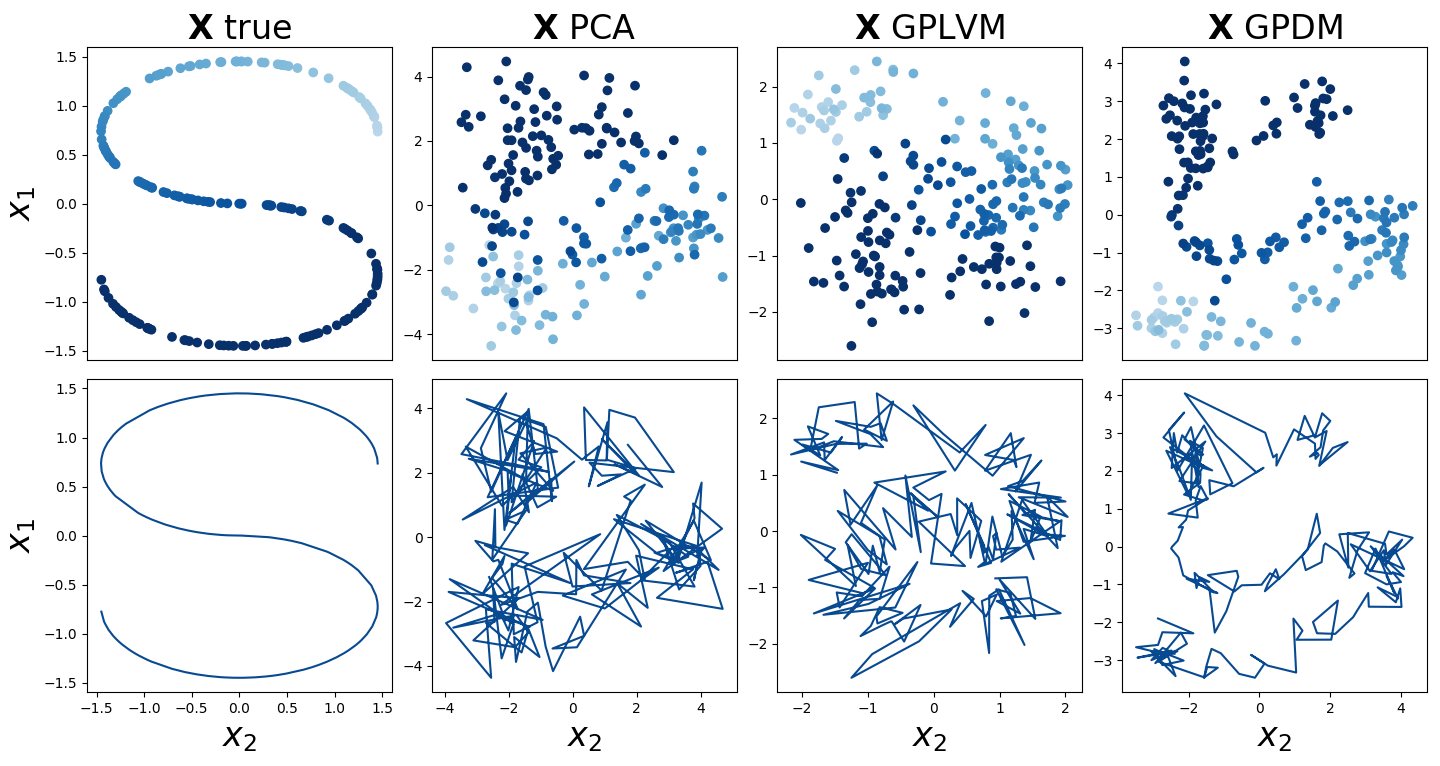
Consider the task of inferring a smooth S-shaped latent variable from high-dimensional observations (Figure $1$, top left). See A1 for Python code to generate this S-shaped variable. Next, let’s fit three dimension reduction techniques to these data: principal component analysis (PCA), GPLVM, and GPDM (Figure $1$, top right three subplots). We find that PCA can uncover the structure at a high-level, but has difficulty disambiguating points in the middle of the S-curve. This makes sense since PCA is a linear model. Both the GPLVM and GPDM do better at inferring the actual S-shape.

Figure 1. (Top row, left) True S-shaped latent variable generated from Scikit-learn's `make_s_curve` function. (Top row, right three plots) The inferred latent variable from three dimension reduction techniques: PCA, GPLVM, and GPDM. (Bottom row) Each subplot is the same as the one above it, but using a line plot rather than a scatter plot.

However, consider the bottom row of plots in Figure $1$. Here, I’ve plotted the latent variables, each $\mathbf{x}_n$, in order using a line plot. This visualization makes it clear that GPDM infers a smoother latent space than the GPLVM. See A2 for Python code to fit a GPDM by optimizing the log posterior.

Appendix

A1. Generating the data

import numpy as np
from   sklearn.datasets import make_s_curve


def gen_data():
    T    = 200
    J    = 40
    X, t = make_s_curve(T)
    X    = np.delete(X, obj=1, axis=1)
    X    = X / np.std(X, axis=0)
    D    = X.shape[1]
    inds = t.argsort()
    X    = X[inds]
    t    = t[inds]
    K    = rbf_kernel(X, 1, 1, 0)
    F    = np.random.multivariate_normal(np.zeros(T), K, size=J).T
    Y    = F + np.random.normal(0, scale=1, size=F.shape)
    return X, Y, t


def rbf_kernel(X, var, length_scale, diag):
    T = len(X)
    diffs = np.expand_dims(X / length_scale, 1) \
          - np.expand_dims(X / length_scale, 0)
    return var * np.exp(-0.5 * np.sum(diffs ** 2, axis=2)) + diag * np.eye(T)

A2. Fitting a GPDM

import autograd.numpy as np
from   autograd import grad
from   scipy.optimize import fmin_l_bfgs_b
from   sklearn.decomposition import PCA


def log_posterior(Y, X, beta, alpha):
    _, J = Y.shape

    K_Y      = rbf_kernel(X, *beta)
    det_term = -J/2 * np.prod(np.linalg.slogdet(K_Y))
    tr_term  = -1/2 * np.trace(np.linalg.inv(K_Y) @ Y @ Y.T)
    LL       = det_term + tr_term

    K_X      = rbf_linear_kernel(X[:-1], *alpha)
    X_bar    = X[1:]
    det_term = -D/2 * np.prod(np.linalg.slogdet(K_X))
    tr_term  = -1/2 * np.trace(np.linalg.inv(K_X) @ X_bar @ X_bar.T)
    LP       = det_term + tr_term

    return LL + LP


def rbf_linear_kernel(X, var, length_scale, diag1, diag2):
    rbf = rbf_kernel(X, length_scale, var, diag1)
    linear = diag2 * X @ X.T
    return rbf + linear


def optimize_gpdm(Y, X0):
    T, D = X0.shape

    beta0 = np.array([1, 1, 1e-6])
    alpha0 = np.array([1, 1, 1e-6, 1e-6])

    def _neg_f(params):
        X = params[:T*D].reshape(X0.shape)
        beta = params[T*D:T*D+3]
        alpha = params[T*D+3:]
        return -1 * log_posterior(Y, X, beta, alpha)

    _neg_fp = grad(_neg_f)
    
    def f_fp(params):
        return _neg_f(params), _neg_fp(params)

    x0 = np.concatenate([X0.flatten(), beta0, alpha0])
    res = fmin_l_bfgs_b(f_fp, x0)
    X_map = res[0][:T*D].reshape(X0.shape)

    return X_map