Lagrange Polynomials

In numerical analysis, given a set of data points $\{(x_n, y_n)\}_{n=1}^{N}$ where each $x_n$ is unique, a Lagrange polynomial (Waring, 1779) is a polynomial of lowest degree that “fits” these data in the sense that the polynomial passes through each point $(x_n, y_n)$. As we will see, the geometric intuition is elegant and the proof of correctness is straightforward. Formally, the Lagrange polynomial is

$L(x) \triangleq \sum_{n=1}^{N} y_n \ell_n(x) \tag{1}$

where each term $\ell_n$ is called a basis polynomial,

$\ell_n(x) \triangleq \prod_{0 \leq m \leq N \\ \;m \neq n} \Big( \frac{x - x_m}{x_j - x_m} \Big).$

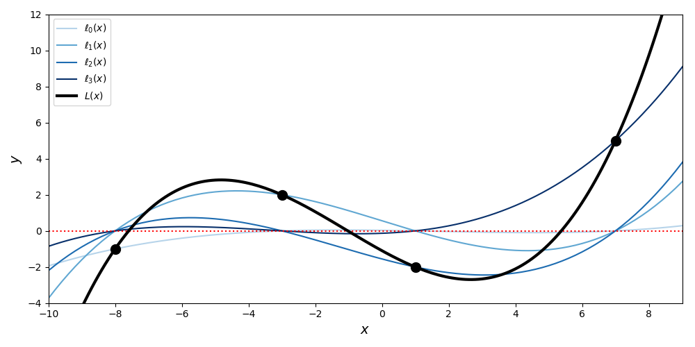
There is a lot of notation to unpack, but the geometric intuition is quite simple (Figure $1$). The Lagrange polynomial $L(x)$ passes through each point because each of the $N$ scaled basis polynomials passes through precisely one of the $N$ points while “zeroing out” at the other points.

Figure 1. An example Lagrange polynomial for $\{(-8, -1), (-3, 2), (1, -2), (7, 5)\}$. The red dashed horizontal line $y = 0$ illustrates how each scaled basis polynomial attains zero for $N - 1$ data points.

To show the correctness of $L(x)$, consider the $k$th basis polynomial on data point $x_n$:

$\ell_k(x_n) = \prod_{0 \leq m \leq N \\ \;m \neq k} \Big( \frac{x_n - x_m}{x_k - x_m} \Big).$

If $k = n$, then each term in the product is one and $\ell_k(x_n) = 1$. If $k \neq n$, then one term in the product is zero, the term in which $x_m = x_n$. Since $k \neq n$, the exclusion $m \neq k$ does not prevent $m = n$. Put differently, $\ell_n(x_n) = 1$, and $\ell_k(x_n) = 0$ provided $k \neq n$. Finally, notice in Equation $1$ that each basis polynomial is scaled by its associated $y_n$.

Why is the Lagrange polynomial the one of least degree that fits $N$ points? To fit $N$ points exactly, we need a polynomial of at most degree $N-1$. Think about it for small $N$. If $N = 2$, we need a line. If $N = 3$, we may need a curve. And so forth. Of course, $N-1$ is the maximum needed degree. For example, three points could form a line in $N = 3$. The Lagrange polynomial has $N$ basis polynomials, each of which has degree $N-1$ because each is the product of $N-1$ terms with a single $x$. So $L(x)$, the sum of $N$ polynomials of degree $N-1$, must have degree at most $N-1$.

Here is the Python implementation that I used to generate Figure $1$:

import numpy as np


class LagrangePoly:

    def __init__(self, X, Y):
        self.n = len(X)
        self.X = np.array(X)
        self.Y = np.array(Y)

    def _basis(self, x, j):
        b = [(x - self.X[m]) / (self.X[j] - self.X[m])
             for m in range(self.n) if m != j]
        return np.prod(b, axis=0)

    def scaled_basis(self, x, j):
        return self._basis(x, j) * self.Y[j]

    def interpolate(self, x):
        b = [self.scaled_basis(x, j) for j in range(self.n)]
        return np.sum(b, axis=0)