Ergodic Markov Chains

An important theorem for Markov chains is the following:

Theorem 1: A Markov chain is ergodic if and only if it has at most one recurrent class and is aperiodic.

This is a very useful theorem. It means that in many cases, we can tell if a Markov chain is ergodic just by analyzing its state diagram. The goal of this post is not to provide a full proof of this theorem. Rather, I want to provide some intuition for why the theorem is true. In particular, the “only if” direction contains an intuitive probabilistic idea called coupling that is worth understanding.

The coupling method was invented by Wolfgang Doeblin (Doeblin, 1939). See A1 for a brief biography of his short but impactful life. Before explaining Doeblin’s idea of coupling, I review Markov chains to introduce notation. This section can be skimmed if one is already familiar with these ideas. Finally, I provide a sketch of a proof of Theorem $1$.

Markov chains

A Markov chain is a powerful mathematical object. It is a stochastic model that represents a sequence of events in which each event depends only on the previous event. Formally,

Definition 1: Let $D$ be a finite set. A random process $X_1, X_2, \dots$ with values in $D$ is called a Markov chain if

$\> \mathbb{P}\{X_{n+1} = x_{n+1} \mid X_n = x_n, \dots, X_0 = x_0\} = \mathbb{P}\{X_{n+1} = x_{n+1} \mid X_n = x_n\}. \tag{1} \>$

We can think of $X_n$ as a random state at time $n$, and the Markovian assumption is that the probability of transitioning from $x_n$ to $x_{n+1}$ only depends on $x_n$. In words, the future depends only on the present. Let $p_{ij}$ be the probability of transitioning from state $i$ to state $j$. A Markov chain can be defined by a transition probability matrix:

Definition 2: The matrix $\mathbf{P} = \big( p_{ij} \big)_{i,j \in D}$ is called the transition probability matrix.

Thus, $\mathbf{P}$ is a $|D| \times |D|$ matrix, where $|D|$ denotes the cardinality of $D$, and the cell value $p_{ij}$ is the probability of transitioning from state $i$ to state $j$, and the rows of $\mathbf{P}$ must sum to one. In this post, we will restrict ourselves to time homogeneous Markov chains:

Definition 3: A Markov chain is called time homogeneous if

$\> \mathbb{P}\{X_{n+1} = j \mid X_n = i\} = p_{ij}, \quad \forall n. \tag{2} \>$

In words, the transition probabilities are not changing as a function of time. Finally, let’s introduce some useful notation for the initial state of the Markov chain. Let

$\mathbb{P}_{x_0}\{\;\cdot\;\} \triangleq \mathbb{P}\{\;\cdot \mid X_0 = x_0\}. \tag{3}$

For example, I will write $\mathbb{P}_a\{X_1 = b\}$ rather than $\mathbb{P}\{X_1 = b \mid X_0 = a\}$. This is because all the conditional probabilities depend on the initial state, and it the usual notation is cumbersome.

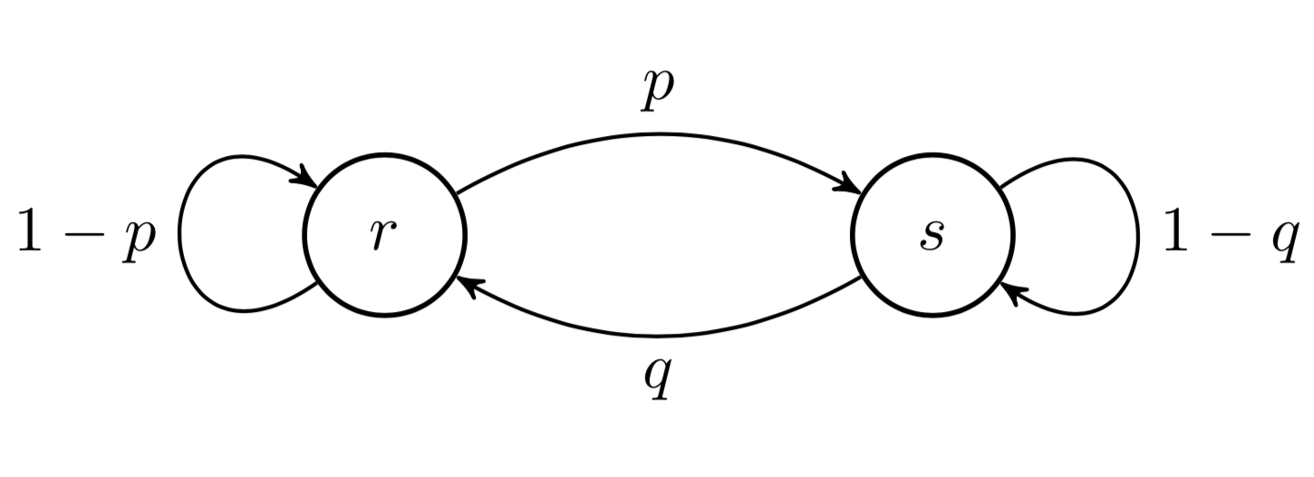
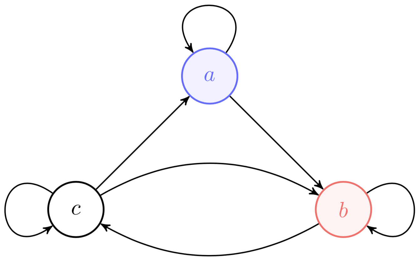
Consider a simple Markov chain modeling the weather. We assume the weather has two states: rainy and sunny. Therefore $D = \{r, s\}$, and $X_n$ is the “weather on day $n$”. The Markov chain model is as follows. If today is rainy ($r$), tomorrow it is sunny ($s$) with probability $p$. If today it is sunny, tomorrow it is rainy with probability $q$. The transition matrix is then

$\mathbf{P} = \begin{array}{|c|cc|} \hline & r & s \\ \hline r & 1 - p & p \\ s & q & 1 - q \\ \hline \end{array}$

and the state diagram of the Markov chain is Figure $1$.

Figure 1: State diagram for a Markov chain with states $D = \{r, s\}$. The probability of moving from $r$ to $s$ is $p$ and from $s$ to $r$ is $q$. The remaining probabilities can be computed because each distribution (row) must sum to unity.

As a consequence of the Markovian assumptions, the probability of any path on a Markov chain is just the multiplication of the numbers along the path. For example, for some Markov chain with states $D = \{a, b, c, d\}$, the probability of a particular path, say $a \rightarrow b \rightarrow b \rightarrow d \rightarrow c$ factorizes as

$\mathbb{P}_a\{X_1 = b, X_2 = b, X_3 = d, X_4 = c\} = p_{ab} \; p_{bb} \; p_{bd} \; p_{dc}. \tag{4}$

You can convince yourself of this easily by repeatedly applying the chain rule and the Markovian assumption (or see A2).

Furthermore, we have an easy formula to compute quantities such as

$\mathbb{P}_i\{X_n = j\} \tag{5}$

for $n \geq 1$. For example, let $n = 2$. Using marginalization and the Markovian assumption, we have

$\begin{aligned} \mathbb{P}_i\{X_2 = j\} &= \sum_{d \in D} \mathbb{P}_i\{X_2 = j, X_1 = d\} \\ &= \sum_{d \in D} \mathbb{P}_i\{X_2 = j \mid X_1 = d\} \mathbb{P}_i\{X_1 = d\} \\ &= \sum_{d \in D} p_{id} \; p_{dj} \end{aligned} \tag{6}$

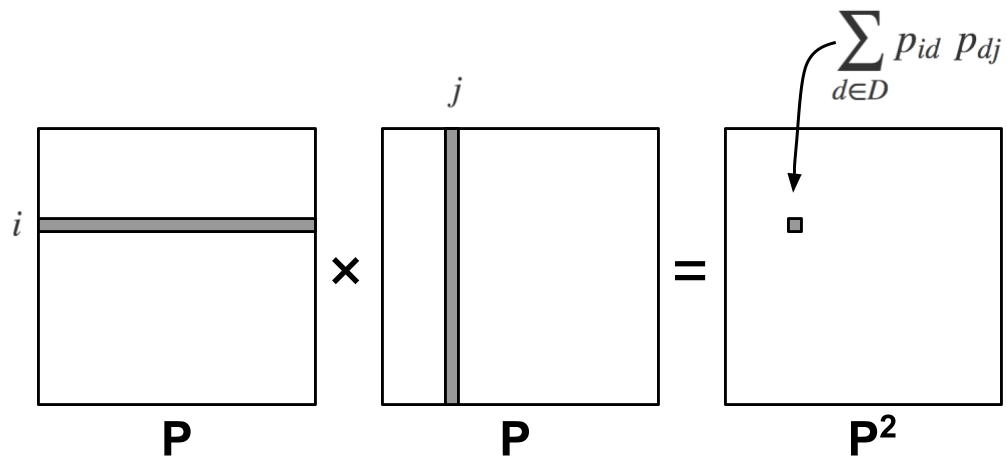
What is this? We are just performing a dot product between the $i$th row and $j$ column of the transition matrix $\mathbf{P}$ (Figure $2$) or

$\mathbb{P}\{X_2 = j \mid X_0 = i\} = \sum_{d \in D} p_{id} \; p_{dj} = \big( \mathbf{P}^2 \big)_{ij}. \tag{7}$

You can check that this idea generalizes so that,

$\mathbb{P}_i\{X_n = j\} = \big(\mathbf{P}^{n}\big)_{ij}. \tag{8}$

Since we are repeatedly applying the transition matrix, $\mathbf{P}^n$ is sometimes called the $n$th iterate of $\mathbf{P}$.

In essence, the dot product performs marginalization, and everything works out nicely because of the Markovian assumption. If the $D$-dimensional vector $\mathbf{v}$ represents a discrete distribution over initial states $X_0$, then $\mathbf{v}^{\top} \mathbf{P}$ is a $D$-dimensional vector representing the probability distribution over $X_1$. This is because a dot product of $\mathbf{v}$ with a single column of $\mathbf{P}$ performs marginalization over $X_0$. If this is unclear, I’d recommend writing out the probabilities explicitly using a small $2 \times 2$ matrix.

Figure 2: The second iterate of $\mathbf{P}$. Since each element $(\mathbf{P}^2)_{ij}$ is the dot product between the $i$th row and $j$th column, the cell values of $\mathbf{P}^2$ represent the probability of starting the Markov chain on state $i$ and arriving at $j$ by $n = 2$.

We are interested in ergodicity, which is a property of a random process in which its time average is the same as its probability space average. Formally,

Definition 4: A Markov chain $\{X_n\}$ is called ergodic if the limit

$\> \boldsymbol{\pi}(j) = \lim_{n \rightarrow \infty }\mathbb{P}_i\{X_n = j\} \tag{9} \>$

exists for every state $j$ and does not depend on the initial state $i$. The $D$-vector $\boldsymbol{\pi}$ is called the stationary probability.

In other words, the probability $\boldsymbol{\pi}(j)$ of being on state $j$ after a long time is independent of the initial state $i$. We can also write this as

$\boldsymbol{\pi}(j) = \lim_{n \rightarrow \infty} (\mathbf{P}^n)_{ij}. \tag{10}$

Consider the following important implication. If a Markov chain is ergodic, then

$\begin{aligned} \boldsymbol{\pi}(j) &\triangleq \lim_{n \rightarrow \infty} (\mathbf{P}^n)_{ij} \\ &\stackrel{\star}{=} \lim_{n \rightarrow \infty} (\mathbf{P}^{n+1})_{ij} \\ &= \lim_{n \rightarrow \infty} (\mathbf{P}^n \mathbf{P})_{ij} \\ &= \lim_{n \rightarrow \infty} \sum_{d \in D} (\mathbf{P}^n)_{id} \mathbf{P}_{dj} \\ &= \sum_{d \in D} \boldsymbol{\pi}(d) \mathbf{P}_{dj}. \end{aligned} \tag{11}$

Step $\star$ holds because if the limit exists, the distinction between $n$ and $n+1$ does not matter. So we can write this as

$\boldsymbol{\pi}^{\top} = \boldsymbol{\pi}^{\top} \mathbf{P}, \tag{12}$

where $\boldsymbol{\pi}$ is a column vector. Hence the name “stationary probability” for $\boldsymbol{\pi}$. It is a distribution that does not change over time.

Since we are interested in ergodicity, let’s now introduce some properties related to reachability and long-term behavior.

Definition 5: We say that $i \leadsto j$ (path from $i$ to $j$) if there is a nonzero probability that starting at $i$, we can reach $j$ at some point in the future.

Definition 6: A state $i$ is called transient if there exists a state $j$ such that $i \leadsto j$ but $j \cancel{\leadsto} i$.

Definition 7: A state $i$ is called recurrent if for all states $j$ that $i \leadsto j$, also $j \leadsto i$.

Intuitively, a transient state is a state that once the chain arrives leaves, it cannot return to; while a recurrent state can be returned to. In other words, these two conditions are opposite. A transient state is not recurrent, and a recurrent state is not transient. Note that if a state is recurrent, every reachable state is also recurrent. We think of a set of recurrent states as a “class” or a “recurrent class”.

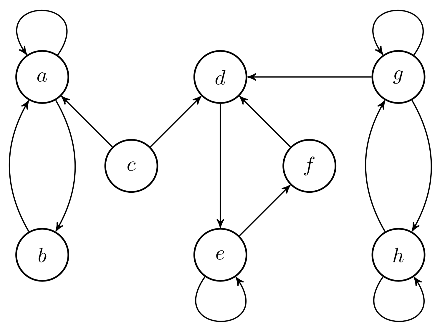
For example, consider Figure $3$. In this Markov chain, states $c$, $g$, and $h$ are transient, while $a$ and $b$ form one recurrent class and $d$, $e$, and $f$ form another.

Figure 3: A Markov chain with $D = \{a, b, c, d, e, f, g, h\}$. The states $c$, $g$, and $h$ are transient, while there are two recurrent classes: $\{a, b\}$ and $\{d, e, f\}$.

As I mentioned in the preamble, defining ergodicity in terms of recurrent states is useful because we can sometimes just look at a Markov chain and know whether it is ergodic, e.g. the Markov chain in Figure $1$ is ergodic, while the Markov chain in Figure $3$ is not. We now have a common framework and notation to tackle Theorem $1$.

Proof sketch

We first show the “if” direction: if a Markov chain is either periodic or containing more than one recurrent class, it cannot be ergodic. We conclude with the “only if” direction, which contains the notion of coupling mentioned in the introduction.

“If” direction

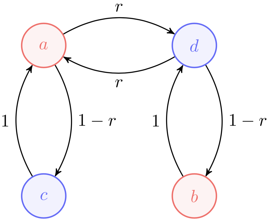
Theorem $1$ implies that there are two blockers to ergodicity. First, if a Markov chain has more than one recurrent class, then it is not ergodic. Second, if a Markov chain is periodic, then it is not ergodic. Consider the Markov chain with two recurrent classes in Figure $4$.

Figure 4: A Markov chain with two recurrent classes, $\{a\}$ and $\{c,d\}$, and a single transient state $b$. The Markov chain cannot be ergodic because the long-term probability of being on a given state depends on the initial state.

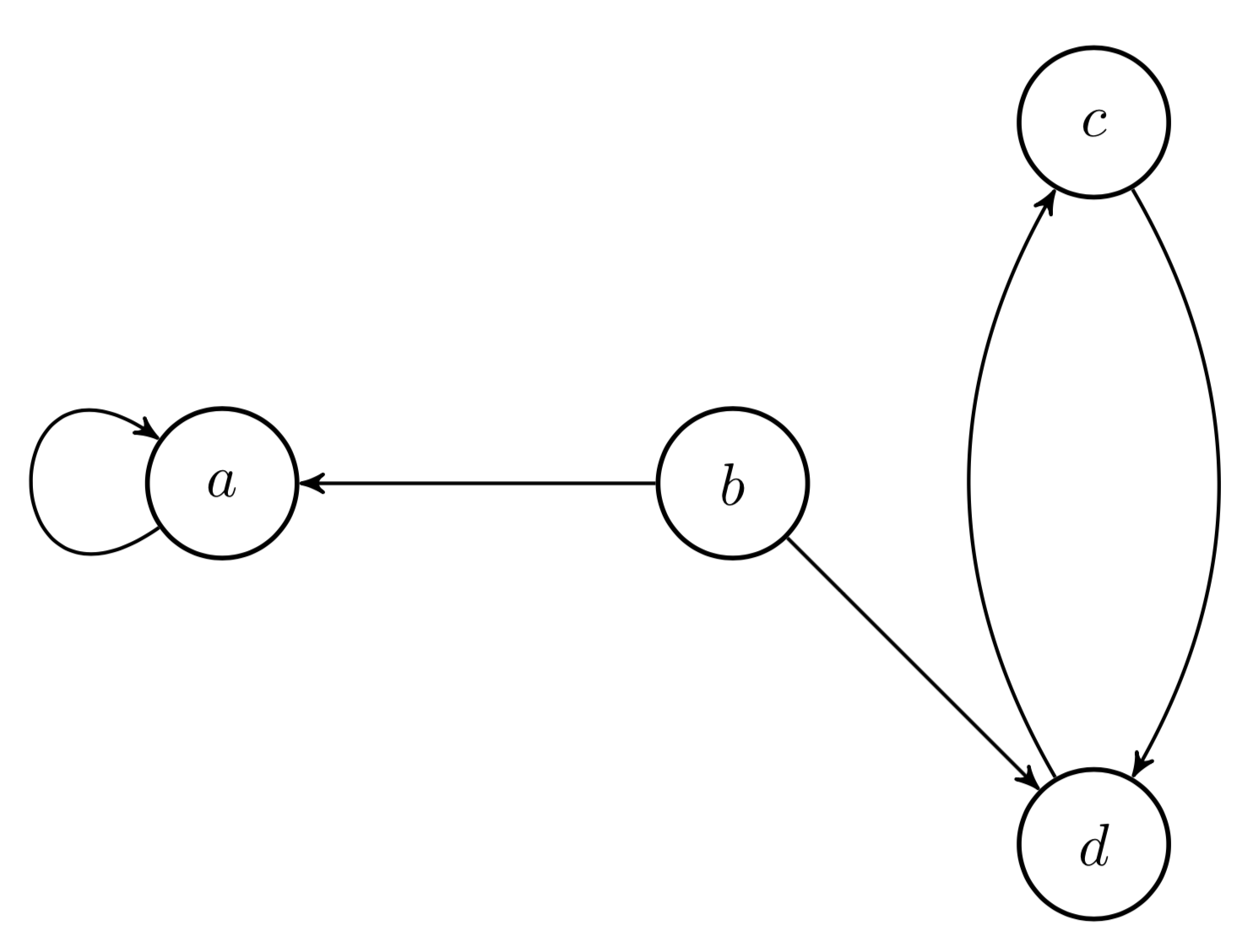
The important thing to note is that it has two recurrent classes. If we start on state $a$, we’ll stay on $a$ forever. If we start in $\{c, d\}$, we’ll stay in this recurrent class forever. If we start on $b$, we’ll end up in one of the two recurrent classes. Therefore, the long-term probability of being on a particular state depends on the initial state. So multiple recurrent classes is an obvious obstruction to ergodicity.

Next, consider the periodic Markov chain in Figure $5$.

Figure 5: A periodic Markov chain with $D = \{a,b,c\}$.

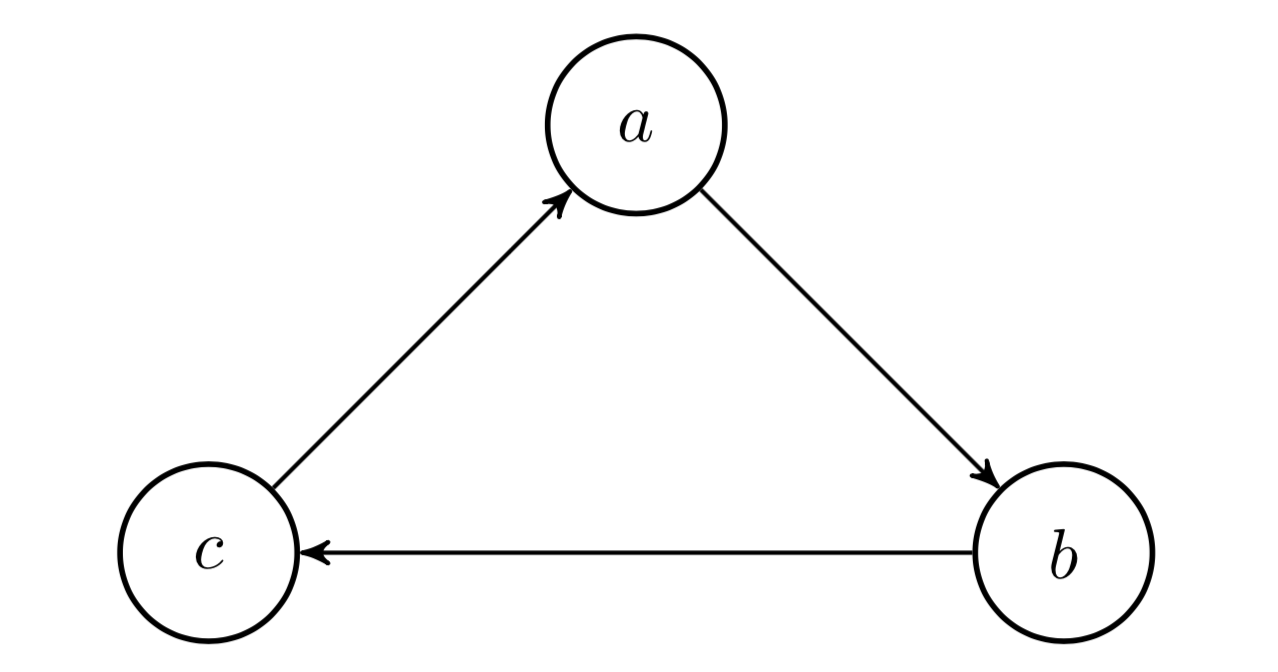
The probability of being on a state by time $n$ is completely dependent upon the initial state. It is easy to see this if we write out two sequences of probability paths side-by-side:

$\begin{aligned} \mathbb{P}_a\{X_0 = a\} = 1 && \mathbb{P}_b\{X_0 = a\} = 0 \\ \mathbb{P}_a\{X_1 = a\} = 0 && \mathbb{P}_b\{X_1 = a\} = 0 \\ \mathbb{P}_a\{X_2 = a\} = 0 && \mathbb{P}_b\{X_2 = a\} = 1 \\ \mathbb{P}_a\{X_3 = a\} = 1 && \mathbb{P}_b\{X_3 = a\} = 0 \\ \mathbb{P}_a\{X_4 = a\} = 0 && \mathbb{P}_b\{X_4 = a\} = 0 \\ \mathbb{P}_a\{X_5 = a\} = 0 && \mathbb{P}_b\{X_5 = a\} = 1 \\ \mathbb{P}_a\{X_6 = a\} = 1 && \mathbb{P}_b\{X_6 = a\} = 0 \\ \mathbb{P}_a\{X_7 = a\} = 0 && \mathbb{P}_b\{X_7 = a\} = 0 \\ \mathbb{P}_a\{X_8 = a\} = 0 && \mathbb{P}_b\{X_8 = a\} = 1 \\ &\qquad\vdots \end{aligned} \tag{13}$

Thus, periodicity is another obstruction to ergodicity, and so both aperiodicity and at most one recurrent class are necessary conditions for ergodicity. If a Markov chain is ergodic, it cannot be periodic or have more than one recurrent class. Perhaps surprisingly, these conditions are also sufficient.

Note that a Markov chain can be periodic even if it is random, meaning even if we cannot predict which state it will go to next given its current state. This is because periodicity refers to the chain being “forced” to switch between sets of states in a predictable manner:

Definition 8: A Markov chain is periodic if its states can be partitioned into $K \geq 2$ periodic classes $S_1, \dots, S_K$ such that $\mathbb{P}\{X_{n+1} \in S_{k+1} \mid X_n \in S_k \} = 1$.

For example, Figure $6$ is a $2$-periodic Markov chain. While a random walk of the chain would be indeed random, we can predict if the chain will be in states $S_1 \triangleq \{a, b\}$ or $S_2 \triangleq \{c, d\}$, conditional on the current set of states.

Figure 6: A $2$-periodic Markov chain with $D = \{a,b,c,d\}$. The chain is periodic since from states $\{a,b\}$ one must always go to states $\{c,d\}$.

“Only if” direction

Let’s assume that we have an aperiodic Markov chain with one recurrent class. We need to show that the Markov chain “forgets” its initial state or

$\lim_{n \rightarrow \infty} \big| \mathbb{P}_i\{X_n = k\} - \mathbb{P}_j\{X_n = k\} \big| = 0 \tag{14}$

for all initial states $i$ and $j$. To see this, we need Wolfgang Doeblin’s idea of coupling. Imagine an aperiodic Markov chain with a single recurrent class in which each state is a lily pad, and imagine that there are two frogs born on two separate lily pads (Figure $7$).

Figure 7: An aperiodic Markov chain with states $D = \{a, b, c\}$ and a single recurrent class re-imagined as a lily pad field. Two frogs begin hopping around on the lily pad field from two different initial states, $a$ and $b$.

Initially, these two frogs hop around independently, moving according to the same transition matrix but with different initial conditions. However, the moment they first land on the same lily pad, they are coupled. That is, at each time, the next state is selected according to the transition probabilities of the Markov chain, and both frogs jump together to the next state. Thus, once they meet, they fall madly in love and go everywhere together. The time at which the frogs meet is the coupling time.

Let’s embrace heteronormativity for ease of notation, and say that one frog is a boy and the other is a girl. The trajectory of the boy frog is $\{B_n\}$ and the girl frog $\{G_n\}$. For example, the movement of the frogs might look something like this,

$\begin{array}{|c|cccccccc|} \hline \text{$n$} & 1 & 2 & 3 & 4 & 5 & 6 & 7 & 8 & \dots \\ \hline \{B_n\} & a & a & a & b & b & c & c & a & \dots \\ \{G_n\} & b & b & c & a & b & c & c & a & \dots \\ \hline \end{array}$

where the coupling time is $n = 5$. On and after $n = 5$, the frogs are linked. Why are we doing this? This is a way of defining two different Markov chains, $\{B_n\}$ and $\{G_n\}$, at two different starting conditions on the same meta-Markov chain $\{X_n\}$. Imagine the boy frog starts on state $a$ and the girl frog state $b$. Then note

$\begin{aligned} \mathbb{P}_a \{X_n = k\} &= \mathbb{P}\{B_n = k\} \\ \mathbb{P}_b \{X_n = k\} &= \mathbb{P}\{G_n = k\}. \end{aligned} \tag{15}$

Recall that $\mathbb{P}(A) = \mathbb{E}[\textbf{1}_{A}]$. It follows that

$\begin{aligned} \big| \mathbb{P}_a \{X_n = k\} - \mathbb{P}_b \{X_n = k\} \big| &= \big| \mathbb{E}[\textbf{1}_{B_n = k}] - \mathbb{E}[\textbf{1}_{G_n = k}] \big| \\ &= \big| \mathbb{E}[\textbf{1}_{B_n = k} - \textbf{1}_{G_n = k}] \big| \\ &\stackrel{\star}{\leq} \mathbb{E}[|\textbf{1}_{B_n = k} - \textbf{1}_{G_n = k}|] \\ &\stackrel{\dagger}{=} \mathbb{E}[\textbf{1}_{B_n \neq G_n}] \\ &= \mathbb{P}(B_n \neq G_n). \end{aligned} \tag{16}$

Step $\star$ holds because of Jensen’s inequality. Step $\dagger$ holds because $\|\mathbf{1}_{B_n = k} - \mathbf{1}_{G_n = k}\| = \mathbf{1}_{B_n \neq G_n}$. If the two indicators on the left-hand side disagree, then the value is one. Otherwise, the value is zero.

This mathematical statement is intuitive: the difference in probability between the two Markov chains $\{B_n\}$ and $\{G_n\}$ is upper bounded by the probability that the two frogs have not yet met. We can drive this difference to zero by showing that $\mathbb{P}(B_n \neq G_n) \rightarrow 0$ as $n \rightarrow \infty$. In words, they will eventually meet. Intuitively, the reason periodicity hurts ergodicity is that it is like the two frogs simply never meet.

So we need to show that the two frogs eventually meet. Note that the pair $\{(B_n, G_n)\}$ is itself a Markov chain but in the state space $\{(i, j): i,j \in \{a,b,c\}\}$. In order to show that the frogs eventually meet, it suffices to show that every state $(i, j)$ where $i \neq j$ is a transient state of the Markov chain $\{(B_n, G_n)\}$. We know that once the two frogs are coupled, they are never uncoupled. That is,

$(k, k) \cancel{\leadsto} (i, j) \tag{17}$

for all $i$ and $j$. Therefore, to show that $(i, j)$ is transient, we just need to show that $(i, j) \leadsto (k, k)$. This is a mathematical formulation of the idea that the frogs eventually meet.

Let $k$ be any recurrent state in the original Markov chain. Since there is only one recurrent class, then we know that $i \leadsto k$ and $j \leadsto k$. If $(i, j) \leadsto (k, k)$ were to fail, we would have a weird situation: even though both frogs can reach $k$ infinitely often, they will never be there at the same time. The only way this can happen is if the frogs are always out of sync, that is: if the chain is periodic.

Therefore, if the original Markov chain has only one recurrent class and is aperiodic, the two frogs must eventually meet in finite time. Thus, as $n \rightarrow \infty$, the Markov chain forgets its initial state and is therefore ergodic.

Acknowledgements

This blog post relies heavily on definitions, notation, and intuition (the story of two frogs) provided by Ramon von Handel in Princeton’s course “Probability and random processes”.

Appendix

A1. Wolfgang Doeblin

Wolfgang Doeblin was a born in Berlin in 1915 to Alfred and Erna Döblin. His father was a famous writer. They were Jewish-German; and Alfred and his family sans Wolfgang fled Berlin a few days after the Reichstag fire in February 1933. Wolfgang stayed behind until April to complete his gymnasium studies. The family was reunited and settled in Paris later that year; and Wolfgang continued his mathematical studies at the Sorbonne.

In the summer of 1936, Doeblin submitted his work on coupling (Doeblin, 1939) for publication. In March 1938, Doeblin defended his thesis—more or less (Doeblin, 1938)—and was drafted into the French army in November. After the start of World War II in September 1939, Doeblin was moved into active duty. In April 1940, Doeblin’s last mathematical note was filed with l’Academie des Sciences by Émile Borel. The note was submitted as a pli cacheté (sealed envelope), which was designed to remain sealed, granting its author intellectual priority if necessary without disclosing the work.

In 1940, Doeblin lost contact with his company while on a mission to the village Housseras. With Nazi troops a few minutes away, Doeblin burned his mathematical notes and took his own life. Doeblin’s pli cacheté was opened in 2000, revealing he had already proven a result (Itô’s lemma) for random processes.

A2. Path probabilities

$\begin{aligned} &\mathbb{P}_a\{X_1 = b, X_2 = b, X_3 = d, X_4 = c\} \\ &= \mathbb{P}_a\{X_4 = c \mid X_1 = b, X_2 = b, X_3 = d\} \mathbb{P}_a \{X_1 = b, X_2 = b, X_3 = d \mid X_0 = a\} \\ &= \mathbb{P}_a\{X_4 = c \mid X_3 = d\} \mathbb{P}_a\{X_1 = b, X_2 = b, X_3 = d\} \\ &= \mathbb{P}_a\{X_4 = c \mid X_3 = d\} \mathbb{P}_a\{X_3 = d \mid X_1 = b, X_2 = b\} \mathbb{P}_a\{X_1 = b, X_2 = b\} \\ &= \mathbb{P}_a\{X_4 = c \mid X_3 = d\} \mathbb{P}_a\{X_3 = d \mid X_2 = b\} \mathbb{P}_a\{X_1 = b, X_2 = b\} \\ &= \mathbb{P}_a\{X_4 = c \mid X_3 = d\} \mathbb{P}_a\{X_3 = d \mid X_2 = b\} \mathbb{P}_a\{X_2 = b \mid X_1 = b\} \mathbb{P}_a\{X_1 = b\} \\ &= p_{ab} \; p_{bb} \; p_{bd} \; p_{dc}. \end{aligned} \tag{A2.1}$