Pólya-Gamma Augmentation

Consider the task of Bayesian inference for models with binomial likelihoods parameterized by log-odds. Two well-known examples of such models are logistic regression and negative binomial regression. For example, in logistic regression, the dependent variables are assumed to be i.i.d. from a Bernoulli distribution with parameter $p$, and therefore the likelihood function is

$\mathcal{L}(p) \propto \prod_{n=1}^{N} p^{y_n} (1 - p)^{1 - y_n} = p^{\sum y_n} (1 - p)^{N - \sum y_n}. \tag{1}$

The observations interact with the response through a linear relationship with the log-odds,

$\log\Big(\frac{p}{1-p}\Big) = \beta_0 + x_1 \beta_1 + x_2 \beta_2 + \dots + x_D \beta_D = \boldsymbol{\beta}^{\top} \mathbf{x}. \tag{2}$

If we solve for $p$ in $(2)$, we get

$p = \frac{\exp(\boldsymbol{\beta}^{\top} \mathbf{x}_n)}{1 + \exp(\boldsymbol{\beta}^{\top} \mathbf{x}_n)} \tag{3}$

and a likelihood of

$\mathcal{L}(\boldsymbol{\beta}) \propto \frac{ [\exp(\boldsymbol{\beta}^{\top} \mathbf{x})]^{\sum y_n} }{ [1 + \exp(\boldsymbol{\beta}^{\top} \mathbf{x})]^{N} }. \tag{4}$

Due to this functional form, Bayesian inference for logistic regression is intractable (Bishop, 2006). This is because the evidence would require normalizing the product of a prior distribution (e.g. a Gaussian prior on $\boldsymbol{\beta}$) times the likelihood function in $(4)$. A similar problem arises for other models with binomial likelihoods parameterized by log-odds. See A1 for a derivation of the likelihood function for negative binomial regression.

However, (Polson et al., 2013) introduced a new method called Pólya-gamma augmentation that allows for constructing simple Gibbs samplers for these models. The goal of this post is to discuss their main results in detail, understand the derivations, and implement this Gibbs sampler.

Pólya-gamma random variables

If $\omega$ is a Pólya-gamma-distributed random variable with parameters $b > 0$ and $c \in \mathbb{R}$, denoted $\omega \sim \text{PG}(b, c)$, then it is equal in distribution to an infinite weighted sum of gamma random variables:

$\omega \stackrel{d}{=} \frac{1}{2 \pi^2} \sum_{k=1}^{\infty} \frac{g_{k}}{(k-1/2)^2 + c^2/(4\pi^2)}. \tag{5}$

Here, $\stackrel{d}{=}$ denotes equality in distribution, and $g_k \sim \text{gamma}(b, 1)$ are independent gamma random variables. Note that this is not the density function. Instead, equality in distribution means that the Pólya-gamma random variable on the left-hand side has the same cumulative distribution function as the random variable on the right-hand side. The density function itself is more complicated (see Polson et al’s first equation in section 2.3).

While a Pólya-gamma random variable’s density function is complicated, Polson et al show that all the finite moments of $\omega$ can be written in closed form. For example, the expectation can be calculated immediately,

$\mathbb{E}[\omega] = \frac{b}{2c} \tanh(c/2). \tag{6}$

In particular, Polson et al proved two useful properties of Pólya-gamma variables. First,

$\frac{(e^{\psi})^a}{(1 + e^{\psi})^b} = 2^{-b} e^{\kappa \psi} \int_{0}^{\infty} e^{- \omega \psi^2 / 2} p(\omega) \text{d}\omega \tag{7}$

where $\kappa = a - b/2$ and $p(\omega) = \text{PG}(\omega \mid b, 0)$. And second,

$p(\omega \mid \psi) \sim \text{PG}(b, \psi). \tag{8}$

While the proof of $(7)$ is a few lines in the paper, it is dense. See A2 for the proof with details. See A3 for a derivation of $(8)$.

Logistic regression with PG augmentation

It may not be immediately obvious why the RHS of $(7)$ is useful. Its utility is that we can construct Gibbs samplers of logistic models or models with likelihoods of the form in $(9)$. To be concrete, consider Bayesian inference for logistic regression. Recall that the $n$-th observation’s contribution to the likelihood $(4)$ is

$\mathcal{L}_n(\boldsymbol{\beta}) = \frac{\big( \exp(\boldsymbol{\beta}^{\top} \mathbf{x}_n) \big)^{y_n}}{1 + \exp(\boldsymbol{\beta}^{\top} \mathbf{x}_n)}. \tag{9}$

Using $(7)$, we can express this likelihood contribution as

$\begin{aligned} \frac{\big( \exp(\boldsymbol{\beta}^{\top} \mathbf{x}_n) \big)^{y_n}}{1 + \exp(\boldsymbol{\beta}^{\top} \mathbf{x}_n)} &= -2 \exp\big\{ \kappa_n \boldsymbol{\beta}^{\top} \mathbf{x}_n \big\} \int_{0}^{\infty} \exp\big\{-\omega_n (\boldsymbol{\beta}^{\top} \mathbf{x}_n)^2 / 2 \big\} p(\omega_n \mid 1, 0) \text{d}\omega_n \tag{10} \\ &= -2 \exp\big\{ \kappa_n \boldsymbol{\beta}^{\top} \mathbf{x}_n \big\} \mathbb{E}_{p(\omega_n \mid 1, 0)}[\exp(- \omega_n(\boldsymbol{\beta}^{\top} \mathbf{x}_n)^2 / 2)], \end{aligned}$

where $\kappa_n = y_n - 1/2$. Note that if we condition on $\omega_n$, the likelihood contribution in $(10)$ is Gaussian in $\boldsymbol{\beta}$:

$\begin{aligned} p(\boldsymbol{\beta} \mid \Omega, y) &= p(\boldsymbol{\beta}) \prod_{n=1}^{N} \mathcal{L}_n(\boldsymbol{\beta} \mid \omega_n) \\ &\stackrel{\ddagger}{\propto} p(\boldsymbol{\beta}) \prod_{n=1}^{N} \exp\big\{ \kappa_n \boldsymbol{\beta}^{\top} \mathbf{x}_n \big\} \exp\big\{-\omega_n (\boldsymbol{\beta}^{\top} \mathbf{x}_n)^2 / 2 \big\} \\ &\stackrel{\star}{\propto} p(\boldsymbol{\beta}) \prod_{n=1}^{N} \exp\Big\{-\frac{\omega_n}{2} \Big( \boldsymbol{\beta}^{\top} \mathbf{x}_n - \frac{\kappa_n}{\omega_n} \Big)^2 \Big\} \\ &= p(\boldsymbol{\beta}) \exp \Big\{ -\frac{1}{2} \big(\mathbf{z} - X \beta \big)^{\top} \Omega \big(\mathbf{z} - X \beta \big) \Big\} \\ &\stackrel{\dagger}{=} p(\boldsymbol{\beta}) \exp \Big\{ -\frac{1}{2} \big( \boldsymbol{\beta} - X^{-1} \mathbf{z}\big)^{\top} X^{\top} \Omega X \big(\boldsymbol{\beta} - X^{-1} \mathbf{z} \big) \Big\} \end{aligned} \tag{11}$

where $\mathbf{z} = \langle \kappa_1 / \omega_1, \dots, \kappa_N / \omega_N \rangle$ and $\Omega = \text{diag}(\omega_1, \dots, \omega_N)$. Step $\ddagger$ holds because the expectation in $(10)$ is constant if we condition on $\omega_n$. Step $\star$ works by completing the square (see A4), while step $\dagger$ is just a little algebra (see A5).

In summary, if our prior on $\boldsymbol{\beta}$ is Gaussian (quadratic in $\boldsymbol{\beta}$), then $(11)$ is tractable because the posterior can be written as Gaussian ($\boldsymbol{\beta}$). This suggests that we can construct a Gibbs sampler, where we repeatedly sample $\Omega$ given $\boldsymbol{\beta}$ and then $\boldsymbol{\beta}$ given $\Omega$.

PG augmented Gibbs sampler

To perform Gibbs sampling with two parameters, we repeatedly fix one parameter while conditionally sampling from the other. Concretely for us, we first initialize $\boldsymbol{\beta}$. Then we for $t = 1, \dots T$, we sample

$\begin{aligned} \Omega^{(t+1)} &\sim p(\Omega \mid \boldsymbol{\beta}^{(t)}) \\ \boldsymbol{\beta}^{(t+1)} &\sim p(\boldsymbol{\beta} \mid \Omega^{(t+1)}). \end{aligned} \tag{12}$

Provided we can compute each density above, we’re done. The first density comes from $(8)$. We know that

$\omega_n \mid \boldsymbol{\beta} \sim \text{PG}(1, \boldsymbol{\beta}^{\top} \mathbf{x}_n). \tag{13}$

In other words, we sample each element along the diagonal of $\Omega$ using $(13)$. The second equation is a bit trickier. If the prior on $\boldsymbol{\beta}$ is $\mathcal{N}(b, B)$, then $p(\boldsymbol{\beta} \mid \Omega, \mathbf{y})$ is

$\boldsymbol{\beta} \mid \Omega, \mathbf{y} \sim \mathcal{N}(\mathbf{m}_{\omega}, V_{\omega}) \tag{14}$

where

$\begin{aligned} V_{\omega} &= (X^{\top} \Omega X + B^{-1})^{-1} \\ \mathbf{m}_{\omega} &= V_{\omega} (X^{\top} \boldsymbol{\kappa} + B^{-1} b) \end{aligned} \tag{15}$

where $\boldsymbol{\kappa} = \langle \kappa_1, \dots, \kappa_N \rangle$. The derivation just requires the matrix formula for completing the square and a bit of algebra (see A6). It is worth skimming this derivation to confirm that the reason it works is because $\boldsymbol{\beta}$ is Gaussian.

Thinking algorithmically, if we can sample $\omega_n$, we can use this reparameterization to get a conditionally Gaussian likelihood centered at $X^{-1} \mathbf{z}$ with covariance $X^{\top} \Omega X$.

Demo

Section 4 of Polson et al discusses simulating PG random variables. The details of this are beyond the scope of this post, and thankfully Scott Linderman has already created a Cython port of Jesse Windle’s code for sampling PG random variables. Using this library, we can easily construct a Gibbs sampler for logistic regression using PG augmentation:

import matplotlib.pyplot as plt
import numpy as np
from   numpy.linalg import inv
import numpy.random as npr
from   pypolyagamma import PyPolyaGamma


def sigmoid(x):
    """Numerically stable sigmoid function.
    """
    return np.where(x >= 0, 
                    1 / (1 + np.exp(-x)),
                    np.exp(x) / (1 + np.exp(x)))

def multi_pgdraw(pg, B, C):
    """Utility function for calling `pgdraw` on every pair in vectors B, C.
    """
    return np.array([pg.pgdraw(b, c) for b, c in zip(B, C)])

def gen_bimodal_data(N, p):
    """Generate bimodal data for easy sanity checking.
    """
    y     = npr.random(N) < p
    X     = np.empty(N)
    X[y]  = npr.normal(0, 1, size=y.sum())
    X[~y] = npr.normal(4, 1.4, size=(~y).sum())
    return X, y.astype(int)


# Set priors and create data.
N_train = 1000
N_test  = 1000
b       = np.zeros(2)
B       = np.diag(np.ones(2))
X_train, y_train = gen_bimodal_data(N_train, p=0.3)
X_test, y_test   = gen_bimodal_data(N_test, p=0.3)
# Prepend 1 for the bias β_0.
X_train = np.vstack([np.ones(N_train), X_train])
X_test  = np.vstack([np.ones(N_test), X_test])

# Peform Gibb sampling for T iterations.
pg         = PyPolyaGamma()
T          = 100
Omega_diag = np.ones(N_train)
beta_hat   = npr.multivariate_normal(b, B)
k          = y_train - 1/2.

for _ in range(T):
    # ω ~ PG(1, x*β).
    Omega_diag = multi_pgdraw(pg, np.ones(N_train), X_train.T @ beta_hat)
    # β ~ N(m, V).
    V         = inv(X_train @ np.diag(Omega_diag) @ X_train.T + inv(B))
    m         = np.dot(V, X_train @ k + inv(B) @ b)
    beta_hat  = npr.multivariate_normal(m, V)

y_pred = npr.binomial(1, sigmoid(X_test.T @ beta_hat))
bins = np.linspace(X_test.min()-3., X_test.max()+3, 100)
plt.hist(X_test.T[y_pred == 0][:, 1],    color='r', bins=bins)
plt.hist(X_test.T[~(y_pred == 0)][:, 1], color='b', bins=bins)
plt.show()

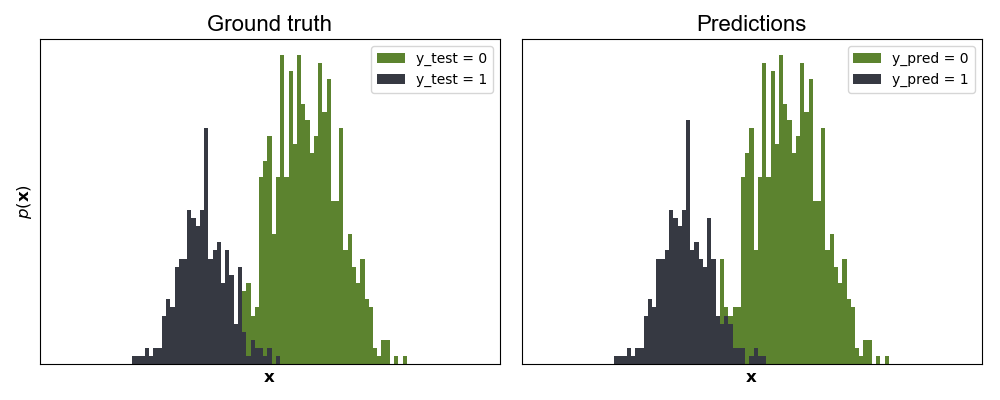
We can see in Figure $1$ that the method works nicely. The only data points that are misclassified are where the two Gaussian distributions overlap.

Figure 1. (Left) Test data from a bimodal distribution colored based on ground truth binary labels. (Right) Test data colored based on predictions from a Bayesianb logistic regression model using PG-augmented Gibb sampling.

Acknowledgements

Thanks to Michael Minyi Zhang for helping with a derivation and finding a bug in my code. Thanks to Yamada Kumpei and Nikos Gianniotis for correcting typos and mistakes. Finally, I asked for a detailed derivation of Polson’s proof on math.stackexchange.com, and Grada Gukovic provided a fantastic answer.

Appendix

A1. Negative binomial likelihood

$\begin{aligned} p(\mathbf{Y} \mid \mathbf{X}, r) &= \prod_{n=1}^{N} {y_{n} + r - 1 \choose y_{n}} p(\mathbf{x}_n)^{r} (1 - p(\mathbf{x}_n))^{y_{n}} \\ &\propto \prod_{n=1}^{N} p(\mathbf{x}_n)^{r} (1 - p(\mathbf{x}_n))^{y_{n}} \\ &= \prod_{n=1}^{N} \Bigg[ \frac{\exp\big(\boldsymbol{\beta}^{\top} \mathbf{x}_n\big)}{1 + \exp\big(\boldsymbol{\beta}^{\top} \mathbf{x}_n\big)} \Bigg]^{r} \Bigg[ 1 - \frac{\exp\big(\boldsymbol{\beta}^{\top} \mathbf{x}_n\big)}{1 + \exp\big(\boldsymbol{\beta}^{\top} \mathbf{x}_n\big)} \Bigg]^{y_{n}} \\ &= \prod_{n=1}^{N} \Bigg[ \frac{\exp\big(\boldsymbol{\beta}^{\top} \mathbf{x}_n\big)}{1 + \exp\big(\boldsymbol{\beta}^{\top} \mathbf{x}_n\big)} \Bigg]^{r} \Bigg[ \frac{1}{1 + \exp\big(\boldsymbol{\beta}^{\top} \mathbf{x}_n\big)} \Bigg]^{y_{n}} \\ &= \prod_{n=1}^{N} \frac{\big[\exp\big(\boldsymbol{\beta}^{\top} \mathbf{x}_n\big)\big]^{r}}{\big[1 + \exp\big(\boldsymbol{\beta}^{\top} \mathbf{x}_n\big)\big]^{y_{n} + r}}. \end{aligned} \tag{16}$

A2. Proof of main result

We want to prove $(7)$ or

$\frac{(e^{\psi})^a}{(1 + e^{\psi})^b} = 2^{-b} e^{\kappa \psi} \int_{0}^{\infty} e^{- \omega \psi^2 / 2} p(\omega) \text{d}\omega$

where $\omega$ is a PG random variable with PDF $(5)$. First, plug $a = \kappa + b/2$ into the LHS of $(7)$,

$\begin{aligned} \frac{(e^{\psi})^a}{(1 + e^{\psi})^b} &= \frac{(e^{\psi})^{\kappa + b/2}}{(1 + e^{\psi})^b} \\ &= \frac{(e^{\psi})^{\kappa} (e^{\psi})^{b/2}}{(1 + e^{\psi})^b} \\ &= \frac{(e^{\psi})^{\kappa}}{(1 + e^{\psi})^b (e^{-\psi/2})^{b}} \\ &= \frac{(e^{\psi})^{\kappa}}{\Big(\frac{1 + e^{\psi}}{e^{\psi/2}}\Big)^{b}} \end{aligned} \tag{17}$

We can introduce the hyperbolic cosine through the identity

$\cosh(x) = \frac{e^{x} + e^{-x}}{2}. \tag{18}$

Plugging $\psi/2$ in for $x$ and working backwards on the denominator in the last line of $(17)$, we have

$\begin{aligned} \Big(\frac{1 + e^{\psi}}{e^{\psi/2}}\Big)^b &= \Big(\frac{e^{\psi}}{e^{\psi/2}} + \frac{1}{e^{\psi/2}}\Big)^b \\ &= \big( e^{\psi/2} - e^{-\psi/2} \big)^2 \\ &= [2 \cosh(\psi/2)]^b. \end{aligned} \tag{19}$

This recapitulates the first step in Polson’s proof, the line starting after the phrase “Appealing to $(3)$, we may write the lefthand side of $(7)$ as…”:

$\frac{(e^{\psi})^a}{(1 + e^{\psi})^b} = \frac{(e^{\psi})^{\kappa}}{\Big(\frac{1 + e^{\psi}}{e^{\psi/2}}\Big)^{b}} = \frac{(e^{\psi})^{\kappa}}{[2 \cosh(\psi/2)]^b} = \frac{2^{-b} (e^{\psi})^{\kappa}}{\cosh^n(\psi/2)}. \tag{20}$

The next step uses $(3)$ from Polson (page $4$):

$\mathbb{E}[\exp(-\omega t)] = \frac{1}{\cosh^b(\sqrt{t/2})} \tag{21}$

and where we just set $t = \psi^2 / 2$:

$\mathbb{E}\Big[\exp\Big(-\omega \frac{\psi^2}{2} \Big)\Big] = \frac{1}{\cosh^b(\psi / 2)}. \tag{22}$

Finally, we plug $(22)$ into $(20)$, and we’re done:

$\frac{(e^{\psi})^a}{(1 + e^{\psi})^b} = \frac{2^{-b} (e^{\psi})^{\kappa}}{\cosh^n(\psi/2)} = 2^{-b} e^{\psi \kappa} \mathbb{E}\Big[\exp\Big(-\omega \frac{\psi^2}{2} \Big)\Big]. \tag{23}$

The expectation is with respect to $\omega \sim \text{PG}(b, 0)$. Just apply the definition of expectation to $(23)$, and we’re done.

A3. Proof of secondary result

By the definitions of a PG random variable and expectation,

$\mathbb{E}[\exp(-\omega) \psi^2/2] = \int_{0}^{\infty} \exp(-\omega \psi^2/2) p(\omega) \text{d}\omega. \tag{24}$

Plug this into Polson’s $(5)$ with $c = \psi$.

A4. Completing the square

This derivation relies on the univariate case of completing the square. If we drop the subscripts and change vectors to scalars to ease notation, we have

$\begin{aligned} \exp\Big\{ \kappa \beta x \Big\} \exp\Big\{ -\omega \frac{(\beta x)^2}{2} \Big\} &= \exp\Big\{ \kappa \beta x - \omega \frac{(\beta x)^2}{2} \Big\} \\ &= \exp\Big\{ -\frac{\omega}{2} \Big( (\beta x)^2 - \frac{2\kappa}{\omega} (\beta x) \Big) \Big\} \\ &= \exp\Big\{ -\frac{\omega}{2} \Big( (\beta x)^2 - \frac{2\kappa}{\omega} (\beta x) + \frac{\kappa^2}{\omega^2} - \frac{\kappa^2}{\omega^2} \Big) \Big\} \\ &\propto \exp \Big\{ -\frac{\omega}{2} \Big( \beta x - \frac{\kappa}{\omega} \Big)^2 \Big\}. \end{aligned} \tag{25}$

A5. Making the likelihood quadratic in $\boldsymbol{\beta}$.

We can show

$\big(\mathbf{z} - X \beta \big)^{\top} \Omega \big(\mathbf{z} - X \beta \big) = \big( \boldsymbol{\beta} - X^{-1} \mathbf{z})^{\top} X^{\top} \Omega X (\boldsymbol{\beta} - X^{-1} \mathbf{z} \big) \tag{26}$

with a little algebra:

$\begin{aligned} &(\mathbf{z} - X \boldsymbol{\beta})^{\top} \Omega (\mathbf{z} - X \boldsymbol{\beta}) \\ &= [X(\boldsymbol{\beta} - X^{-1} \mathbf{z})]^{\top} \Omega [X(\boldsymbol{\beta} - X^{-1} \mathbf{z})] \\ &= (\boldsymbol{\beta} - X^{-1} \mathbf{z})^{\top} X^{\top} \Omega X (\boldsymbol{\beta} - X^{-1} \mathbf{z}). \end{aligned} \tag{27}$

A6. Sum of two quadratic forms in $\mathbf{x}$

Note that the sum of two quadratic forms in $\mathbf{x}$ can be written as a single quadratic form plus a constant term that is independent of $\mathbf{x}$. Consider the equation

$(\mathbf{x} - \boldsymbol{\mu})^{\top} \Sigma^{-1} (\mathbf{x} - \boldsymbol{\mu}) + (\mathbf{x} - \boldsymbol{\nu})^{\top} \Psi^{-1} (\mathbf{x} - \boldsymbol{\nu}). \tag{28}$

First, expand each quadratic term out:

$\begin{aligned} (\mathbf{x} - \boldsymbol{\mu})^{\top} \Sigma^{-1} (\mathbf{x} - \boldsymbol{\mu}) &= \mathbf{x}^{\top} \Sigma^{-1} \mathbf{x} - 2 \boldsymbol{\mu}^{\top} \Sigma^{-1} \mathbf{x} + \boldsymbol{\mu}^{\top} \Sigma^{-1} \boldsymbol{\mu} \\ (\mathbf{x} - \mathbf{\nu})^{\top} \Psi^{-1} (\mathbf{x} - \mathbf{\nu}) &= \mathbf{x}^{\top} \Psi^{-1} \mathbf{x} - 2 \boldsymbol{\nu}^{\top} \Psi^{-1} \mathbf{x} + \boldsymbol{\nu}^{\top} \Psi^{-1} \boldsymbol{\nu}. \end{aligned} \tag{29}$

If we combine “similar” terms and distribute, we get

$\begin{aligned} \mathbf{x}^{\top}(\Sigma^{-1} + \Psi^{-1}) \mathbf{x} - 2(\boldsymbol{\mu}^{\top} \Sigma^{-1} + \boldsymbol{\nu}^{\top} \Psi^{-1}) \mathbf{x} + (\boldsymbol{\mu}^{\top} \Sigma^{-1} \boldsymbol{\mu} + \boldsymbol{\nu}^{\top} \Psi^{-1} \boldsymbol{\nu}) \end{aligned} \tag{30}$

which is again quadratic in $\mathbf{x}$. If we set

$\begin{aligned} V &= \Sigma^{-1} + \Psi^{-1} \\ \mathbf{m} &= \Sigma^{-1} \boldsymbol{\mu} + \Psi^{-1} \boldsymbol{\nu} \\ R &= \boldsymbol{\mu}^{\top} \Sigma^{-1} \boldsymbol{\mu} + \boldsymbol{\nu}^{\top} \Psi^{-1} \boldsymbol{\nu} \end{aligned} \tag{31}$

and apply completing the square, then we can write the above as

$\begin{aligned} &\mathbf{x}^{\top} V \mathbf{x} - 2 \mathbf{m}^{\top} \mathbf{x} + R \\ &= (\mathbf{x} - V^{-1} \mathbf{m}) V (\mathbf{x} - V^{-1} \mathbf{m}) - \mathbf{m}^{\top} \mathbf{V}^{-1} \mathbf{m} + R. \end{aligned} \tag{32}$

This is proportional to a Gaussian kernel with mean $V^{-1} \mathbf{m}$ and covariance $V^{-1}$. We can ignore the remainder terms $\mathbf{m}^{\top} \mathbf{V}^{-1} \mathbf{m}$ and $R$ since they does not depend on $\boldsymbol{\beta}$.

This is the trick used in the paper. Using the notation in the paper, both Gaussians are quadratic in $\boldsymbol{\beta}$; one has mean $\mathbf{b}$ and covariance $B$, and the other has mean $X^{-1} \mathbf{z}$ and covariance $X^{\top} \Omega^{-1} X$. Doing a little pattern matching, we get

$\begin{aligned} V &= (B^{-1} + X^{\top} \Omega X)^{-1} \\ \mathbf{m} &= B^{-1} \mathbf{b} + (X^{\top} \Omega X) X^{-1} \mathbf{z} \\ &= B^{-1} \mathbf{b} + X^{\top} \Omega \mathbf{z} \\ &\stackrel{\star}{=} B^{-1} \mathbf{b} + X^{\top} \boldsymbol{\kappa}. \end{aligned} \tag{33}$

Step $\star$ holds because if we multiply each value in $\boldsymbol{\Omega}$s by the definition of $\mathbf{z}$, we get back $\boldsymbol{\kappa}$. Thus, we have shown that $(\boldsymbol{\beta} \mid y, \omega)$ is Gaussian with mean $V^{-1} \mathbf{m}$ and covariance $V^{-1}$.