Random Noise and the Central Limit Theorem

Gaussian noise is ubiquitous in modeling. For example, Bayesian linear regression, probabilistic PCA, Bayesian matrix factorization, and many signal processing models all assume some additive noise term $\boldsymbol{\epsilon} \sim \mathcal{N}(\boldsymbol{\mu}, \boldsymbol{\Sigma})$ for some model-specific $\boldsymbol{\mu}$ and $\boldsymbol{\Sigma}$. But why do we assume that random noise is Gaussian? There are two answers to this question. First, the Gaussian distribution has some very nice analytic properties. For example, the sum of two independent Gaussian random variables is also Gaussian and a linear map on a Gaussian distribution produces another Gaussian distribution. But second, the Central Limit Theorem motivates the idea that random noise will most likely be Gaussian. When I first heard this second justification, it was not immediately clear why. The goal of this post is to describe the Central Limit Theorem in detail and then explain how it relates to assuming random noise is Gaussian distributed.

The Central Limit Theorem

The Central Limit Theorem (CLT) is arguably one of the most important ideas in probability and statistics because its implications are widespread. The CLT states that, under certain conditions, the sampling distribution of a normalized sum of independent random variables, themselves not necessarily normally distributed, tends towards a normal distribution. There is a lot in that sentence, and it is worth unpacking slowly. In various research conversations, I have heard people casually evoke the CLT as meaning that “everything is Gaussian”, but this is a little sloppy. The statement is more precise, with important implications in that precision.

First, let us formalize things. Let $X_i$ denote the $i$th draw of a random variable. Note that $X_i$ is the random variable before sampling, meaning it is still a random variable and not fixed. And let $S_n$ be a random variable representing the average of $n$ such draws:

$S_n = \frac{X_1 + X_2 + \dots + X_n}{n}$

The CLT’s claim is not about an $X_i$ but rather $S_n$ after normalization.

There are many different variants of the CLT. For example, the De Moivre–Laplace theorem is a special case of the CLT. For simplicity, I begin with the first one presented on Wikipedia, the self-contained Lindeberg–Lévy CLT (Lindeberg, 1922), which states

Lindeberg–Lévy CLT: Suppose $\{ X_1, X_2, \dots \}$ is a sequence of i.i.d. random variables with $\mathbb{E}[X_i] = \mu$ and $\text{Var}[X_i] = \sigma^2 < \infty$. Then as $n$ approaches infinity, the random variables $\sqrt{n}(S_n − \mu)$ converge in distribution to a normal $\mathcal{N}(0, \sigma^2)$.

But what is this random variable $\sqrt{n}(S_n − \mu)$? Didn’t we just say that the CLT is about $S_n$? To see the connection, let’s do a little manipulation. First, since $\mathbb{E}[X_i] = \mu$, then

$\begin{aligned} \mathbb{E}[S_n] &= \mathbb{E} \left[ \frac{X_1 + X_2 + \dots + X_n}{n} \right] \\ &= \frac{n \mathbb{E}[X_i]}{n} \\ &= \mu \end{aligned}$

So the term $(S_n - \mu)$ is simply mean-centering the random variable $S_n$.

And what is the variance of $S_n$? Note that for independent random variables $X$ and $Y$, $\text{Var}(X + Y) = \text{Var}(X) + \text{Var}(Y)$. This makes sense. Since the random variables are uncorrelated, the total variance—our total uncertainty about what values they might each take—is the sum of variances. And if $\alpha$ is a scalar, then $\alpha^2 \text{Var}(X) = \text{Var}(\alpha X)$. So

$\begin{aligned} \text{Var}(S_n) &= \text{Var} \left( \frac{X_1 + X_2 + \dots + X_n}{n} \right) \\ &= \sum_{i=1}^{n} \text{Var} \left( \frac{X_i}{n} \right) \\ &= \sum_{i=1}^{n} \frac{1}{n^2} \text{Var} (X_i) \\ &= \frac{\text{Var} (X_i)}{n} \\ &= \frac{\sigma^2}{n} \end{aligned}$

Now if you want to normalize a Gaussian random variable to be $\mathcal{N}(0, 1)$ distributed, you need to mean center the random variable and divide by the standard deviation:

$\frac{(S_n - \mu)}{\sqrt{\frac{\sigma^2}{n}}} = \frac{\sqrt{n} (S_n - \mu)}{\sigma}$

And this random variable is distributed as

$\lim_{n \rightarrow \infty} \frac{\sqrt{n} (S_n - \mu)}{\sigma} \stackrel{d}{\rightarrow} \mathcal{N}(0, 1)$

which is equivalent to the Lindeberg–Lévy CLT.

I think it’s worth mentioning why the Lindeberg–Lévy CLT takes the form it does, namely that the random variable $\sqrt{n} (S_n - \mu)$ approaches $\mathcal{N}(0, \sigma^2)$. First, while $S_n$ and $n S_n$ are both approximately Gaussian distributed, their means and variances are functions of $n$, and therefore these two random variables do not converge to a particular distribution. Furthermore, my guess is that the Lindeberg–Lévy CLT mentions converging to $\mathcal{N}(0, \sigma^2)$ rather than $\mathcal{N}(0, 1)$ because it makes clear that this normalized random variable $\sqrt{n} (S_n - \mu)$ converges to a Gaussian distribution with the same variance as the original random variable.

Intuition for the CLT

Now that we know what the CLT claims, we can play with it a little bit. (I typically start with intuition, but in this case, I found that defining things really helped me understand which random variable was Gaussian distributed.) The CLT claims that if we draw $n$ i.i.d. random variables from a wide class of distributions with a first moment $\mu$ and second moment $\sigma^2 < \infty$, the random variable $\sqrt{n} (S_n - \mu)$ is $\mathcal{N}(0, \sigma^2)$ distributed. Let’s empirically test this.

For this experiment, let’s use the uniform distribution, $\mathcal{U}(a, b)$. First, let’s look at the distribution of $S_n$ where each $X_i \sim \mathcal{U}(a, b)$. The reason we want to look at $S_n$ rather than $\sqrt{n} (S_n - \mu)$ is that it is easier to see the Gaussian distribution “peaking” if it is un-normalized (Figure $1$).

Figure 1. For each $n$, we draw a uniformly distributed random variable $X_i \sim \mathcal{U}(0, 5)$ and compute the sum $S_n = \frac{1}{n} \sum_{i=1}^{n} X_i$. We sample a new $S_n$ ten thousand times for each $n$ and then compute the histogram of the variables $S_n$.

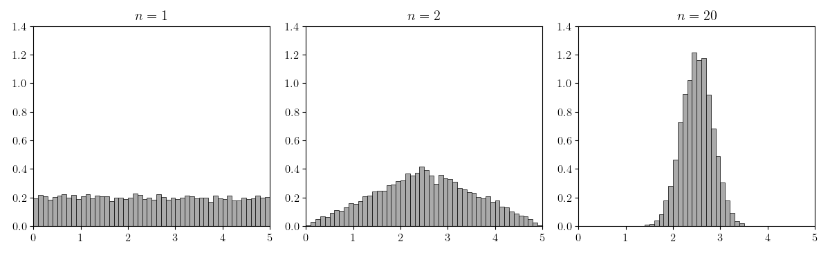
In Figure $1$, we can see that when $n = 1$, the histogram looks like the uniform distribution. But as $n$ increases, the histogram of the random variable $S_n$ looks more and more Gaussian distributed. The minimal example in Python to generate this figure is in the Appendix.

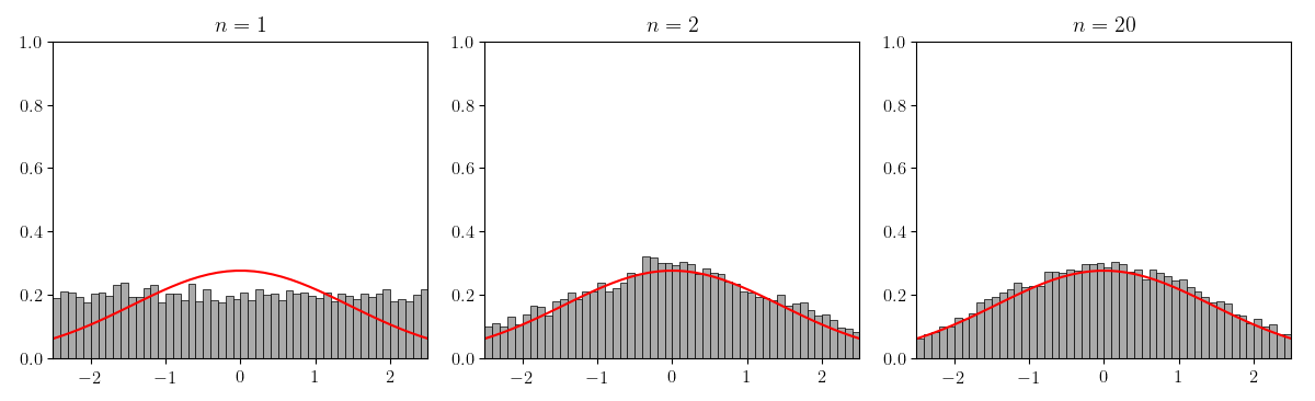
Of course, Figure $1$ does not precisely demonstrate what is stated in the Lindeberg–Lévy CLT. We really should normalize $S_n$ and verify that $\sqrt{n}(S_n - \mu)$ converges to $\mathcal{N}(0, \sigma^2)$ for the normal distribution with second moment $\frac{1}{12}(a-b)^2$ (Figure $2$).

Figure 2. Demonstration of the CLT. For each $n$, we draw a uniformly distributed random variable $X_i \sim \mathcal{U}(0, 5)$ and compute the normalized sum $\sqrt{n} (S_n - \mu)$. We compute a new $\sqrt{n} (S_n - \mu)$ ten thousand times for each $n$ and then compute the histogram of the variables $S_n$. The red curve is the distribution $\mathcal{N}(0, \sigma^2)$ where $\sigma^2 = \frac{1}{12} (5 - 0)^2$.

The Lyapunov CLT

Lindeberg–Lévy CLT has two conditions for our random variables. The random variables must (1) be i.i.d. and (2) have finite variance. If either of these conditions is not met, the CLT is not guaranteed to hold. For example, consider the Cauchy distribution, which is pathological in the sense that both its first and second moments are undefined, i.e. $\sigma^2 \nless \infty$. If you take the code in the Appendix and re-run it with np.random.standard_cauchy, you will find that $S_n$ is not Gaussian distributed.

But it is noteworthy that while the samples must be independent, they need not be identically distributed. After reading the Lindeberg–Lévy CLT, I assumed the data must be identically distributed, but I could not convince myself why. To understand my thinking, consider some sequence of random variables,

$X_1 + Y_2 + Y_3 + X_4 + \dots + X_n$

where $X_i$ and $Y_i$ denote differently distributed random variables. If we just re-order these random variables and re-number them, we get:

$X_1 + X_2 + \dots + X_m + Y_1 + Y_2 + \dots + Y_k$

where $m$ is the number of $X_i$ samples and $k$ is the number of $Y_i$ samples. Clearly by the Lindeberg–Lévy CLT, the sums $X_1 + X_2 + \dots X_m$ and $Y_1 + Y_2 + \dots + Y_k$ are Gaussian distributed, and since these random variables are independent, their sums must be Gaussian distributed. After some searching, I realized that this has already been proven and is the Lyapunov CLT which states that the random variables $X_i$ must be independent but not necessarily identically distributed.

In my mind, this is an important generalization for understanding why noise is so often modeled as Gaussian distributed.

Additive Gaussian noise

Now that we understand the Lyapunov CLT, the assumption that noise is Gaussian starts to make sense. Noise is not one thing but rather the byproduct of interference from potentially many different sources. Let’s think of an example. Imagine a Bluetooth speaker receiving a signal from your laptop. In this context, noise can be many things: a microwave oven with a similar radio frequency, sensor errors due to overheating, physical interference as you pick up the speaker, and so on. Each of these sources of noise can be thought of as interferring with or being added to the true signal from your laptop. And while these sources of noise are neither Gaussian distributed nor identically distributed in general, their total effect can be plausibly modeled as a single Gaussian random variable—or additive Gaussian noise.

Appendix

1. Code to generate Figure 1

import numpy as np
import matplotlib.pyplot as plt

a = 0
b = 5
reps = 2000
fig, axes  = plt.subplots(1, 3)

for n, ax in zip([1, 2, 20], axes.flat):
    rvs = [np.random.uniform(a, b, n).mean() for _ in range(reps)]
    ax.hist(rvs, density=True)
plt.show()